Bring this project to life
When building machine learning models, we are always looking for the most efficient parameters for our models and training configurations. These settings might range from optimizers to batch sizes, layer stack setup, and even data shape.
In this article, we’ll discuss batch sizing constraints one may come across while training a neural network architecture. We'll also see how this element can be affected by the GPU's power and it's available memory. Then we'll take a look at what can be done to find the perfect batch size for our GPU/Model combination.
Understanding the terminology
Sample
A sample represents a single element of data. It includes inputs for the training algorithm as well as outputs for calculating the errors by comparing to the prediction. It can also be called: observation, an input vector, or a feature vector.
Batch size
The batch size refers to the quantity of samples used to train a model before updating its trainable model variables, or weights and biases. That is, a batch of samples is passed through the model at each training step and then passed backward to determine the gradients for each sample. In order to determine the updates for the trainable model variables, the gradients of all samples are then averaged or added, depending on the type of optimizer that is used. This process will be repeated for the subsequent batch of samples when the parameters have been updated.
Epoch
The number of epochs, which is a hyperparameter that controls how many times the learning algorithm will run through the full training Dataset.
One epoch indicates that the internal model parameters have had a chance to be updated one time for each sample in the training Dataset. Depending on the configuration, there can be one or more batches within a single epoch.
Iteration
An iteration is simply the number of batches needed to complete a single epoch. For example, if a Dataset contains 10000 samples divided into 20 batches. Then, we would need a number of 500 iterations ( 10 000 = 500 × 20 ) to go through one epoch.
Identifying the effect of batch size on training
GPU usage and memory
First, let's evaluate the effect of varying batch size on GPU usage and GPU memory. Machine learning researchers at the University of Ohio practically evaluated the effect of increasing batch size on the GPU utilization. They used 3 of the most used machine learning frameworks (TensorFlow, PyTorch and MXnet) then recorded the results:
TensorFlow:
| Batch size | 4 | 8 | 16 | 32 | 64 | 128 | 256 | 512 | 1024 |
|---|---|---|---|---|---|---|---|---|---|
| GPU Usage (%) | 5.65% | 5.65% | 29.01% | 30.46% | 36.17% | 30.67% | 24.88% | 22.45% | 22.14% |
| GPU Memory usage(MB) | 694.274 | 665.804 | 649.137 | 620.909 | 694.563 | 641.000 | 541.333 | 535.063 | 535.063 |
PyTorch:
| Batch size | 4 | 8 | 16 | 32 | 64 | 128 | 256 | 512 | 1024 |
|---|---|---|---|---|---|---|---|---|---|
| GPU Usage (%) | 9.59% | 9.98% | 11.46% | 11.00% | 13.29% | 13.00% | 9.91% | 11.00% | 9.67% |
| GPU Memory usage(MB) | 520.222 | 516.784 | 509.296 | 530.000 | 495.250 | 502.642 | 503.478 | 525.818 | 553.524 |
MXNet:
| Batch size | 4 | 8 | 16 | 32 | 64 | 128 | 256 | 512 | 1024 |
|---|---|---|---|---|---|---|---|---|---|
| GPU Usage (%) | 22.13% | 24.65% | 30.22% | 33.14% | 34.91% | 34.83% | 38.33% | 46.09% | 46.09% |
| GPU Memory usage(MB) | 502.452 | 505.479 | 536.672 | 606.953 | 720.811 | 2495.153 | 2485.639 | 2491.920 | 2511.472 |
These results were then plotted in graphs for comparison
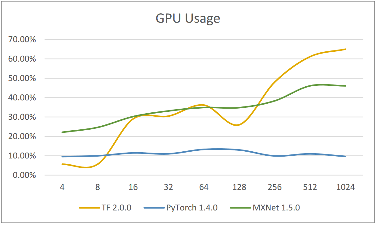
We see that TensorFlow's GPU usage is the lowest and MXnet's GPU utilization is largest when batch size is relatively small. While, TensorFlow has the highest GPU utilization rate and PyTorch has the lowest when batch sizes are relatively large. Furthermore, we can also observe that as batch sizes grow, GPU consumption will grow dramatically as well.
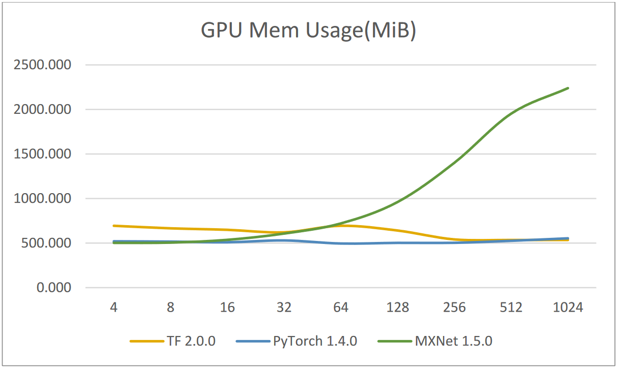
When the batch size increases, we can see that MXnet takes up substantially more memory than the other two do, although they barely change. Most of the time, MXnet takes up the most memory. The fact that MXnet saves all batch size data in the GPU RAM and then releases them once the entire application has run through is one potential explanation. On the other hand, batch data processing is how TensorFlow and PyTorch operate. Data relative to a single batch will be removed from the memory after processing for a single epoch.
Increasing batch size is a straightforward technique to boost GPU usage, though it is not always successful. The gradient of the batch size is often computed in parallel on the GPU. Therefore, a big batch size can boost the GPU usage and training performance as long as there is enough memory to accommodate everything. In the case of PyTorch, GPU and memory utilization remain essentially unchanged. This is because PyTorch employs a method of distribution that can decrease GPU utilization, CPU memory, and training speed when the batch size is too high, and vice versa.
Generally speaking, memory consumption increases with higher batch size values.
The framework used, the parameters of the model and the model itself as well as each batch of data affect memory usage. However, this effect is majorly dependent on the model used!
Accuracy and algorithm performance
The same academic paper included some other interesting findings about the batch size and its effect on the trained algorithm accuracy. The researchers evaluated, for the TensorFlow framework, the accuracy after 10 epochs for different values of the batch size:
| Batch size | 4 | 8 | 16 | 32 | 64 | 128 | 256 | 512 | 1024 |
|---|---|---|---|---|---|---|---|---|---|
| Accuracy after 10 epochs | 32.55% | 45.83% | 63.06% | 68.59% | 68.97% | 69.77% | 64.82% | 57.28% | 51.02% |
Then we can plot this variation in the graph below:

When evaluating the accuracy, employing various batch size values may have important repercussions that should be taken into account when selecting one. Using small or high batch sizes could have two main negative effects.

Over-fitting
Bad generalization may result from large batch sizes and models can even get stuck in a local minima. The neural network will perform pretty well on samples outside of the training set thanks to generalization. However the opposite can also happen, the neural network can perform poorly on samples found outside of the training set, which is essentially over-fitting. This effect is seen in the graph; beginning with batch size 256, the model deviates from the absolute minimum and performs with lower accuracy on fresh data. A study on large-batch training for deep learning examined the same phenomenon analytically and confirmed the findings.
Under-fitting (Slow convergence)
Small batch sizes may be to blame for the learning algorithm's slow convergence. The variable updates that were performed in each phase and calculated using a batch of samples will decide the beginning point for the future batch of samples. Because each step involves the random selection of training samples from the training set, the gradients produced are noisy estimates based on incomplete data. The less data we use in a single batch, the noisier and less precise the gradient estimations are. In other words, when the batch size is small, a single sample has a bigger influence on the applied variable updates. To put it in another way, smaller batch sizes may cause the learning process to be noisier and more irregular, thereby delaying the learning process. In the example above, we can see that batch size of 4 was only able to get us to an accuracy of 32% after 10 epochs which is not as good as the accuracy obtained for batch size 128.
How to maximize the batch size
As discussed in the preceding section, batch size is an important hyper-parameter that can have a significant impact on the fitting, or lack thereof, of a model. It may also have an impact on GPU usage. We can expect that raising the batch size will boost training speed (i.e. GPU utilization), but this gain will be limited by the aforementioned convergence issues (over-fitting).
So, in this section, we'll go over some strategies for determining the optimal batch size that takes advantage of everything a GPU has to offer while avoiding the extreme situation of over-fitting.
Data augmentation
One of the techniques that could be considered is data augmentation. This method would offer the possibility of increasing the batch size while keeping a good and acceptable accuracy increase per each epoch. Although the application of this technique varies by area, it usually requires increasing the data set by making carefully controlled changes to the training data. In the case of image recognition, for example, the training set can be enlarged by translating, rotating, shearing, resizing, cropping and even flipping the images in the training data.
Conservative Training
The convergence rate for some optimizers is better that others in case of large batch training. Studies on the effect of stochastic optimization techniques showed that the convergence rate of the standard Stochastic Gradient Descent (SGD) optimizer can be improved, especially for the large batches. A method based on an approximate optimization of a conservatively regularized objective function within each mini batch was introduced in the previously mentioned paper. Additionally, the research demonstrated that the convergence rate is not affected by the size of the mini batch. They also showed that we could outperform traditional SGD with the right implementations of alternative optimizers, like ADAM, for instance. The ADAM optimization approach is a stochastic gradient descent extension that has lately gained more popularity for deep learning applications especially in computer vision and natural language processing.
Robust Training
Robust training is another natural technique to prevent the consequences of bad generalization when increasing batch size. These strategies try to decrease the effect of increasing batch size by maximizing a worst-case (Robust) cost rather than the nominal cost of the objective function.
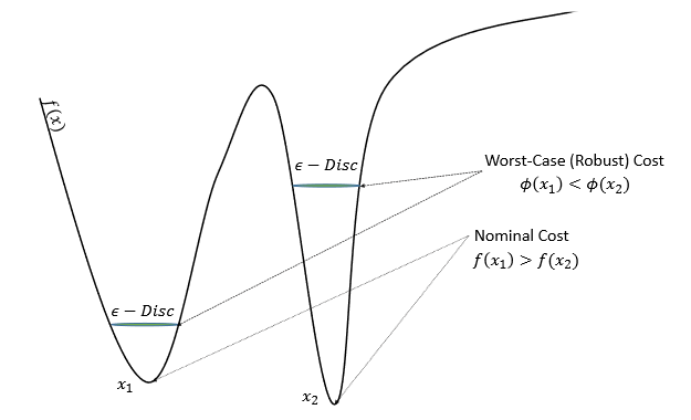
In the preceding example, the maximum robust worst-case is positioned differently than the objective function's nominal minimal location.
Case study: Cats and dogs images classification
In this section, we will build a classifier for images of cats and dogs using TensorFlow/Keras. The model's performance is then evaluated for various batch size values, with a standard SGD optimizer and the default data format. Then, using the strategies previously discussed, we'll try to increase the batch size while keeping or even improving the accuracy.
Bring this project to life
Let's start by preparing the Dataset
Download & Unzip
curl https://download.microsoft.com/download/3/E/1/3E1C3F21-ECDB-4869-8368-6DEBA77B919F/kagglecatsanddogs_5340.zip --output dataset.zip
7z x dataset.zip
Split training/validation/testing subsets
First, we create folders for storing the resized images
mkdir -p train/Cat
mkdir -p train/Dog
mkdir -p validation/Cat
mkdir -p validation/Dog
mkdir -p test/Cat
mkdir -p test/Dog
Then, using Keras image preprocessing library, we load the images, resize them into 200px per 200px files then save the resulting in the folders. We take a total of 1000 image per class: 600 for training, 200 for validation and 200 for testing.
# importing libraries
from keras.preprocessing.image import load_img,save_img,ImageDataGenerator
from os import listdir
from tensorflow import keras

# load dogs vs cats dataset, reshape into 200px x 200px image files
classes = ['Cat','Dog']
photos, labels = list(), list()
files_per_class = 1000
for classe in classes:
  i = 0
  # enumerate files in the directory
  for file in listdir('PetImages/'+classe):
    if file.endswith(".jpg"):
      # determine class
      output = 0.0
      if classe == 'Dog':
        output = 1.0
      # load image
      photo = load_img('PetImages/'+classe +'/' + file, target_size=(200, 200))
      if i < 600:
        save_img('train/'+classe+'/'+file, photo)
      elif i < 800:
        save_img('validation/'+classe+'/'+file, photo)
      else:
        save_img('test/'+classe+'/'+file, photo)
      i = i + 1
      if i == files_per_class:
        break
Training & evaluating the model
For the model, we will use Tensorflow/Keras sequential model. The training and evaluation processes are embedded in a function that takes as input the batch size and the optimizer. This function will be later used for evaluating the effect of the optimizer on the batch size
def get_accuracy_for_batch_size(opt, batch_size):
  print("Evaluating batch size " + str(batch_size))
  # prepare iterators
  datagen = ImageDataGenerator(rescale=1.0/255.0)
  train_it = datagen.flow_from_directory(directory='train/',
    class_mode='binary', batch_size=batch_size, target_size=(200, 200))
  val_it = datagen.flow_from_directory(directory='validation/',
    class_mode='binary', batch_size=batch_size, target_size=(200, 200))
  test_it = datagen.flow_from_directory('test/',
    class_mode='binary', batch_size=batch_size, target_size=(200, 200))

  # create model
  model = keras.Sequential()
  model.add(keras.layers.Conv2D(32, (3, 3), activation='relu', kernel_initializer='he_uniform', padding='same', input_shape=(200, 200, 3)))
  model.add(keras.layers.MaxPooling2D((2, 2)))
  model.add(keras.layers.Flatten())
  model.add(keras.layers.Dense(128, activation='relu', kernel_initializer='he_uniform'))
  model.add(keras.layers.Dense(1, activation='sigmoid'))

  # compile model
  model.compile(optimizer=opt, loss='binary_crossentropy', metrics=['accuracy'])

  # train the model
  model.fit(train_it,
                      validation_data = train_it,
                      steps_per_epoch = train_it.n//train_it.batch_size,
                      validation_steps = val_it.n//val_it.batch_size,
                      epochs=5, verbose=0)

  # evaluate model
  _, acc = model.evaluate(test_it, steps=len(test_it), verbose=0)
  return acc
Comparing optimizers: SGD vs Adam
For different values of the batch size (16, 32, 64 and 128), we will evaluate the accuracy of the model after 5 epochs, for both cases of Adam and SGD optimizers.
batch_size_array = [16,32,64,128]
accuracies_sgd = []
optimizer = "sgd"
for bs in batch_size_array:
  accuracies_sgd.append(get_accuracy_for_batch_size(optimizer, bs))

accuracies_adam = []
optimizer = "adam"
for bs in batch_size_array:
  accuracies_adam.append(get_accuracy_for_batch_size(optimizer, bs))
Then, we'll plot the results using Matplotlib
import matplotlib.pyplot as plt
plt.plot(batch_size_array, accuracies_sgd, color='green',label='SGD')
plt.plot(batch_size_array, accuracies_adam, color='red',label='Adam')
plt.show()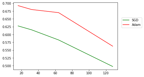
We can clearly see that for batch size 16, the SGD have an accuracy around 62%, which starts to decline rapidly as soon as we increase the batch size. This is not the case with Adam, the accuracy decline is not as steep, around batch size 64 the accuracy is still in the neighborhood of 67% which represents a four fold increase while still maintaining an acceptable accuracy.
But, we can also notice that for both optimizers, starting from batch size 128 the accuracy decreases drastically. So, we can deduce that the optimal batch size for Adam with this model is 64 and 16 for SGD.
Effect of data augmentation
Let's start by creating new directories for the augmented training and validation data.
!mkdir -p train_augmented/Cat
!mkdir -p train_augmented/Dog
!mkdir -p validation_augmented/Cat
!mkdir -p validation_augmented/Dog
Now, let's fill these folders with the original data and a new resized and cropped version for each image. This will result in a final Dataset with double the size of the original one. The said manipulation is also done through the image preprocessing Keras library:
from tensorflow import image
# load dogs vs cats dataset, reshape into 200x200 files
classes = ['Cat','Dog']
photos, labels = list(), list()
files_per_class = 1000
for classe in classes:
  i = 0
  # enumerate files in the directory
  for file in listdir('PetImages/'+classe):
    if file.endswith(".jpg"):
      # determine class
      output = 0.0
      if classe == 'Dog':
        output = 1.0
      # load image
      photo = load_img('PetImages/'+classe +'/' + file, target_size=(200, 200))
      photo_resized = photo.resize((250,250))
      photo_cropped = photo_resized.crop((0,0, 200, 200))
      if i < 600:
        save_img('train_augmented/'+classe+'/'+file, photo)
        save_img('train_augmented/'+classe+'/augmented_'+file, photo_cropped)
      elif i < 800:
        save_img('validation_augmented/'+classe+'/'+file, photo)
        save_img('validation_augmented/'+classe+'/augmented_'+file, photo_cropped)
      else:
        save_img('test/'+classe+'/'+file, photo)
      i = i + 1
      if i == files_per_class:
        break
Now we introduce a new training and evaluation function that takes as input the training/validation folders as well as the batch size. This function will use the Adam optimizer for all cases of Datasets.
def get_accuracy_for_batch_size_augmented_data(train_folder,validation_folder, batch_size):
  print("Evaluating batch size " + str(batch_size))
  # prepare iterators
  datagen = ImageDataGenerator(rescale=1.0/255.0)
  train_it = datagen.flow_from_directory(directory=train_folder,
    class_mode='binary', batch_size=batch_size, target_size=(200, 200))
  val_it = datagen.flow_from_directory(directory=validation_folder,
    class_mode='binary', batch_size=batch_size, target_size=(200, 200))
  test_it = datagen.flow_from_directory('test/',
    class_mode='binary', batch_size=batch_size, target_size=(200, 200))

  # create model
  model = keras.Sequential()
  model.add(keras.layers.Conv2D(32, (3, 3), activation='relu', kernel_initializer='he_uniform', padding='same', input_shape=(200, 200, 3)))
  model.add(keras.layers.MaxPooling2D((2, 2)))
  model.add(keras.layers.Flatten())
  model.add(keras.layers.Dense(128, activation='relu', kernel_initializer='he_uniform'))
  model.add(keras.layers.Dense(1, activation='sigmoid'))

  # compile model
  model.compile(optimizer="adam", loss='binary_crossentropy', metrics=['accuracy'])

  # train the model
  model.fit(train_it,
                      validation_data = train_it,
                      steps_per_epoch = train_it.n//train_it.batch_size,
                      validation_steps = val_it.n//val_it.batch_size,
                      epochs=5, verbose=0)

  # evaluate model
  _, acc = model.evaluate(test_it, steps=len(test_it), verbose=0)
  return acc
Then, we will evaluate the accuracy for different batch sizes. In both cases of the original data and then the augmented Dataset.
batch_size_array = [16,32,64,128,256]
accuracies_standard_data = []
for bs in batch_size_array:
  accuracies_standard_data.append(get_accuracy_for_batch_size_augmented_data("train/","validation/", bs))

accuracies_augmented_data = []
for bs in batch_size_array:
  accuracies_augmented_data.append(get_accuracy_for_batch_size_augmented_data("train_augmented/","validation_augmented/", bs))
Finally, we plot the resulting accuracy values for both Datasets. You may run out of memory on a free GPU, so consider upgrading to our Pro or Growth plan's to access even more powerful GPUs on Paperspace.
import matplotlib.pyplot as plt
plt.plot(batch_size_array, accuracies_standard_data, color='green',label='Standard data')
plt.plot(batch_size_array, accuracies_augmented_data, color='red',label='Augmented data')
plt.legend(bbox_to_anchor =(1.25, 0.8))
plt.show()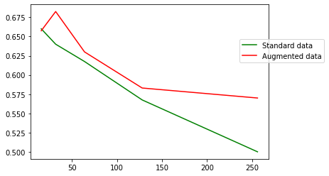
Using the augmented data, we can increase the batch size with lower impact on the accuracy. In fact, only with 5 epochs for the training, we could read batch size 128 with an accuracy of 58% and 256 with an accuracy of 57.5%.
As a result of combining these two strategies (Adam optimizer and Data augmentation), we were able to employ a batch size of 128 instead of 16, which is an 8-fold gain, while keeping an acceptable accuracy percentage.
Conclusion
In this article, we talked about batch sizing restrictions that can potentially occur when training a neural network architecture. We have also seen how the GPU's capability and memory capacity might influence this factor. Then, we evaluated the effect of batch size increase on the model accuracy. Finally, we investigated how to determine the ideal batch size for our GPU/Model combination.
There is often the existence of a threshold beyond which the quality of the model degrades as the batch size used for model training is increased. However, with some right methodologies, as demonstrated in the case study, this degradation may be conveyed to larger batch sizes, allowing us to increase this parameter and make better use of the existing GPU capabilities.
Resources
https://etd.ohiolink.edu/apexprod/rws_etd/send_file/send?accession=osu1587693436870594
https://arxiv.org/pdf/1711.00489.pdf