If you are a fan of Google translate or some other translation service, do you ever wonder how these programs are able to make spot-on translations from one language to another on par with human performance. Well, the underlying technology powering these super-human translators are neural networks and we are going build a special type called recurrent neural network to do French to English translation using Google's open-source machine learning library, TensorFlow.
Note: This tutorial assumes some beginner to intermediate level understanding of python, neural networks, natural language processing, TensorFlow and Jupyter notebook.
Most of the code from this tutorials is from the TensorFlow documentation page.
Bring this project to life
Before we start building our network, let's take a look at an overview of this article.
- We’ll start by describing how to load and preprocess our dataset for the task.
- Then we’ll move on to explain what a sequence to sequence model is and its importance in solving the translation problem.
- We’ll then describe what an attention mechanism is and the problems it helps solve.
- We’ll wrap this article up by bringing all we've discussed together to build our translation model
Let us begin first by loading and getting our data ready for training.
Data loading and pre-processing stage
Personally, building an efficient data input pipeline for a Natural Language Processing task is one of the most tedious stages in the whole NLP task. Since our task is to translate a piece of text from one language into another language, we are going to need our corpus in a parallel corpus structure. Luckily for us, the dataset we are going use is arranged in this structure. Let’s download our dataset and examine it. (source: manythings.org).
!wget https://www.manythings.org/anki/fra-eng.zip
!unzip  fra-eng.zip
The above snippet is going download our zipped dataset and unzip it. We should obtain two files in our workspace directory: fra.txt which is the main file we are going to use and _about.txt (not important). Let’s see how our fra.txt file is structured. We can do so by using the snippet below.
with open("fra.txt",'r') as f:
        lines = f.readlines()
print(lines[0])
This block of code outputs:
output[]: 'Go.\tVa !\n'We are only looking at the first line of our corpus. As displayed, it consists of an English word, phrase or sentence and a french word, phrase or sentence separated by a tab. ‘\n’ indicates that the next pair of English and French sentences is on a new line.As a next step, we are going build a class for each language that is going to map each word in a language to a unique integer number. This is important since computers only understand numbers instead of strings and characters. This class is going to have three dictionary data structures, one to map each word to a unique integer, one to map an integer to a word and the third, to map a word to its total number in the corpus. The class is going to have two important functions to add words from the corpus to their class dictionaries. Let’s take a look at how to do this.
class Lang(object):
    def __init__(self, name):
        self.name = name
        self.word2int = {} #maps words to integers
        self.word2count = {} #maps words to their total number in the corpus
        self.int2word = {0 : "SOS", 1 : "EOS"} #maps integers to tokens (just the opposite of word2int but has some initial values. EOS means End of Sentence and it's a token used to indicate the end of a sentence. Every sentence is going to have an EOS token. SOS means Start of Sentence and is used to indicate the start of a sentence.)
        self.n_words = 2 #Intial number of tokens (EOS and SOS)

    def addWord(self, word):
        if word not in self.word2int:
            self.word2int[word] = self.n_words
            self.word2count[word] = 1
            self.int2word[self.n_words] = word
            self.n_words += 1

        else:
            self.word2count[word] += 1

    def addSentence(self, sentence):
        for word in sentence.split(" "):
            self.addWord(word)
In our class, the addWord function just adds a word as a key to the word2int dictionary with its value being a corresponding integer. The opposite is done for the int2word dictionary. Note that we keep track of how many times we’ve come across a word when parsing our corpus to populate the class dictionaries and if we’ve already come across a particular word, we desist from adding it to the word2int and int2word dictionaries and instead keep track of how many times it appears in our corpus using the word2count dictionary.What addSentence does is to simply iterate through each sentence and for each sentence, it splits the sentence into words and implements the addWord function on each word in each sentence.
Our corpus consists of French words which may have some characters like ‘Ç’. For simplicity sake, we convert them into their normal corresponding ASCII characters(Ç → C). Also we create white spaces between words and punctuation attached to these words . (hello’s → hello s). This is to ensure that the presence of a punctuation does not create two words for a particular word (difference integers would be assign to “they’re” and they are). We can achieve both of these with the snippet below.
def unicodeToAscii(s):
    return "".join(c for c in unicodedata.normalize("NFD", s) \
                   if unicodedata.category(c) != "Mn")
def normalizeString(s):
    s = unicodeToAscii(s.lower().strip())
    s = re.sub(r"([!.?])", r" \1", s)
    s = re.sub(r"[^a-zA-Z?.!]+", " ", s)
    return s
Let’s combine these two helper functions to load the dataset as a list of list containing the pair of sentences.
def load_dataset():
    with open("/content/gdrive/My Drive/fra.txt",'r') as f:
        lines = f.readlines()

    pairs = [[normalizeString(pair) for pair in
              line.strip().split('\t')] for line in lines]
    return pairs

pairs = load_dataset()
A portion of the list of pairs should look like this
pairs[856:858]
out[]: [['of course !', 'pour sur .'], ['of course !', 'mais ouais !']]
To reduce the training time for our demonstration, we are going to filter out our dataset to remove sentences with more than ten words. We can achieve that with the functions below which iterates through our pairs and removes pairs which have sentences containing more than ten words.
MAX_LENGTH = 10
def filterPair(p):
    return len(p[0].split()) < MAX_LENGTH and \
len(p[1].split()) < MAX_LENGTH

def filterPairs(pairs):
    return [pair for pair in pairs if filterPair(pair)]
Our neural network is going to run on a computer and computers only understand numbers but our dataset is made of strings. We need to find a way to convert our dataset of strings into numbers and if you can recall, earlier, we built a Language class which maps words to numbers using a dictionary data structure. Let’s create a helper function that will take as parameters a sentence and the language instance corresponding to the sentence(i.e for an English sentence, we use the English language instance) and encode the sentence into numerical values that the computer understands.
def sentencetoIndexes(sentence, lang):
    indexes = [lang.word2int[word] for word in sentence.split()]
    indexes.append(EOS_token)
"""
Iterates through a sentence, breaks it into words and maps the word to its corresponding integer value using the word2int dictionary which we implemented in the language class
"""
    return indexes
As a next step, we are going to populate the word2int dictionary in each Language class with words and assign a corresponding integer to each word in a new function. Also since we are going to batch our dataset, we are going to apply padding to sentences with words less than the maximum length we proposed. Let’s see how to do this.
def build_lang(lang1, lang2, max_length=10):
    input_lang = Lang(lang1)
    output_lang = Lang(lang2)
    input_seq = []
    output_seq = []

    for pair in pairs:
"""Iterates through the list of pairs and for each pair, we implement the addSentence function on the English sentence using the English Languuage class. The same is done to the corresponding French sentence"""
        input_lang.addSentence(pair[1])
        output_lang.addSentence(pair[0])
    for pair in pairs:
"""
We convert each sentence in each pair into numerical values using the sentencetoIndexes function we implemented earlier.
"""
        input_seq.append(sentencetoIndexes(pair[1], input_lang))
        output_seq.append(sentencetoIndexes(pair[0], output_lang))
    return keras.preprocessing.sequence.pad_sequences(input_seq, maxlen=max_length, padding='post', truncating='post'), \
keras.preprocessing.sequence.pad_sequences(output_seq, padding='post', truncating='post'), input_lang, output_lang

input_tensor, output_tensor, input_lang, output_lang = build_lang('fr', 'eng')
Let’s take a look at what our build function returns.
print("input_tensor at index 10: {}".format(input_tensor[10]))
print("output_tensor at index 10: {}".format(output_tensor[10]))
print("corresponding integer value for 'nous' {}".format(input_lang.word2int['nous']))
print("corresponding integer value for 'she' {}".format(output_lang.word2int['she']))
output: [] input_tensor at index 10: [10 18 3 1 0 0 0 0 0 0]
output_tensor at index 10: [13 6 1 0 0 0 0 0 0 0]
corresponding integer value for 'nous' 97
corresponding integer value for 'she' 190
Our data is now ready to fed into a neural network but to accelerate our training process, we’ll have to sort our dataset into batches. TensorFlow data API provides us with tools to perform this task.
BUFFER_SIZE = len(input_tensor)
dataset = tf.data.Dataset.from_tensor_slices((input_tensor, output_tensor)).shuffle(BUFFER_SIZE)
dataset = dataset.batch(16)
We are now all set to build our model.
Sequence to Sequence models
There are several architectures of Recurrent Neural Networks, each suited for a particular group of tasks. Some examples are many-to-one architecture for task such as sentiment analysis and one-to-many for music generation but we are going to employ the many-to-many architecture which is suited for tasks such as chat-bots and of course Neural Machine Translation.
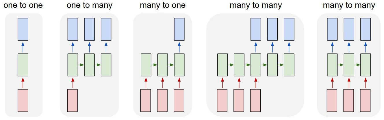
As you can see from the image above, there are two types of many-to-many architectures but we are going to use the first one which consist of two networks: one to take in the input sentence and the other to translate into another language in the case of machine translation. This architecture is suitable for our task because we have inputs and outputs with different lengths. This special class of architecture is called a Sequence to Sequence model. The network where the input is encoded is called the Encoder. The other network is called the decoder since it receives a fixed size vector from the encoder to decode the outputs.t sentence. The minds behind this architecture are Ilya Sutskever, Oriol Vinyals and Quoc V. Le. Link to paper: https://arxiv.org/pdf/1409.3215.pdf
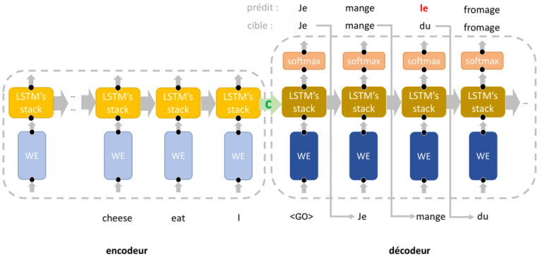
You probably may have noticed a drawback in this architecture. If you haven’t, it’s cool. Let’s go ahead and discuss this drawback. From the diagram immediately above, we can observe that the only information that the decoder receives from the encoder is the hidden state indicated in the diagram. This hidden state is a fixed size vector into which the encoder squeezes every bit of information about the input sentence and passes it on to the decoder to generate the output sentence. This might work fairly well for shorter sentences but this fixed size vector tends to become a bottleneck for longer sentences. This is where attention mechanism becomes a crucial part of our translation network.
Attention Mechanism
Later that same year when Sutskever and his team proposed their sequence to sequence architecture, several efforts were made to surmount the bottleneck in Sutskever’s model. One major breakthrough that caught the attention of many was the work of Yoshua Bengio and some others in the paper titled Neural Machine Translation by Jointly Learning to Align and Translate. The basic idea behind this architecture is that whenever the decoder is generating a particular output word, it considers information about all the words in the input sentence and determines which words in the inputs sentence are relevant to generate the correct output word. In a sequence model, the common way to pass information about the data at a particular time-step to the next time-step is through the hidden states. This means each hidden state at a particular time-step in our model has some information about the word at that time-step. It does make sense that not every word in the input sentence is required to generate a particular word in the output sentence. For example, when we humans want to translate the french sentence "Je suis garcon" to "I am a boy", obviously when we are translating the word "boy", intuitively we would be paying more attention to the word "garcon" than any other word in our input french sentence. That is exactly how attention mechanism in a sequence to sequence model works - our decoder pays attention to a particular word or group of words when generating a particular word. You probably might be wondering how our decoder network pays attention to words. Well it uses connections or weights. The greater the connection or weight to a particular word in the input sentence, the more our decoder is paying attention to that word. We also ought to know that our weights should be a function of the hidden state immediately before the time step we are decoding ( this gives the decoder information about already decoded words) and the encoder outputs but we don’t know what that function is so we let back-propagation take over to learn the appropriate weights. We also ensure that all weights mapping all words in the input sentence to a particular word in the output sentence add up to one. This is asserted using a softmax function. Now that we have some basic idea of attention mechanism, let’s go ahead and implement our model. We’ll start with the encoder. (Does not employ attention mechanism).
Encoder
The Encoder is usually very easy to implement. It’s made up of two layers: the Embedding layer which converts each token(word) into a dense representation and a Recurrent Network layer(We are going to use a Gate Recurrent Unit Network for simplicity).
class Encoder(keras.models.Model):
    def __init__(self, vocab_size, num_hidden=256, num_embedding=256, batch_size=16):
        super(Encoder, self).__init__()
        self.batch_size = batch_size
        self.num_hidden = num_hidden
        self.num_embedding = num_embedding
        self.embedding = keras.layers.Embedding(vocab_size, num_embedding)
        self.gru = keras.layers.GRU(num_hidden, return_sequences=True,
                                    recurrent_initializer='glorot_uniform',
                                   return_state=True)

    def call(self, x, hidden):
        embedded = self.embedding(x) #converts integer tokens into a dense representation
        rnn_out, hidden = self.gru(embedded, initial_state=hidden)
        return rnn_out, hidden
    def init_hidden(self):
        return tf.zeros(shape=(self.batch_size, self.num_hidden))
Readers should take note of two very important parameters in the GRU implementation: return_sequences and return_state. return_sequences ensures that the GRU outputs the hidden state of each time step. Remember that we need this information to access information about each word in the input sequence. Return state returns the hidden state of the last time step. We need this tensor to be used as initial hidden state for the decoder.
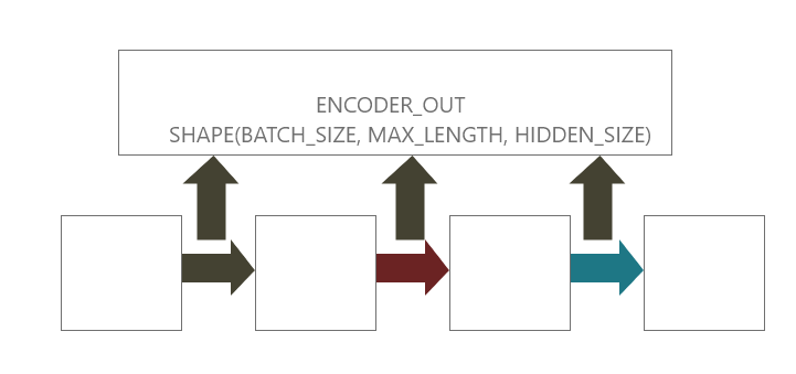
In the call function where forward propagation of our network is implemented. we first pass the input tensor through an embedding layer and then through a GRU layer. This returns the RNN output(rnn_out) of shape (batch_size, max_sequence length, hidden_size) and hidden state of shape (batch_size, hidden_size).
Decoder
Unlike the Encoder, the Decoder is a bit complex. It has in addition to the Embedding and Gated Recurrent Network layer an Attention layer and a fully connected layer. Let’s first see how to implement the attention layer.
class BahdanauAttention(keras.models.Model):
    def __init__(self, units):
        super(BahdanauAttention, self).__init__()

        self.W1 = keras.layers.Dense(units)
        self.W2 = keras.layers.Dense(units)
        self.V = keras.layers.Dense(1)

    def call(self, encoder_out, hidden):
        #shape of encoder_out : batch_size, seq_length, hidden_dim (16, 10, 1024)
        #shape of encoder_hidden : batch_size, hidden_dim (16, 1024)

        hidden = tf.expand_dims(hidden, axis=1) #out: (16, 1, 1024)

        score = self.V(tf.nn.tanh(self.W1(encoder_out) + \
                                  self.W2(hidden))) #out: (16, 10, 1)

        attn_weights = tf.nn.softmax(score, axis=1)

        context =  attn_weights * encoder_out #out: ((16,10,1) * (16,10,1024))=16, 10, 1024
        context = tf.reduce_sum(context, axis=1) #out: 16, 1024
        return context, attn_weights
It seems pretty simple to implement but you really need to pay attention to the dimensions as data moves through the pipeline. The call function where forward propagation takes place takes in two parameters; encoder_out which represents all the hidden states at each timestep in the encoder and hidden which represents the hidden state before the current timestep where we are generating the correct word.
Since the hidden is the hidden state of a timestep in the decoder, we add a dimension of size 1 to represent the timestep hence shape of hidden becomes (batch_size, time_step, hidden_size). Earlier, I mentioned that the weights for determining attention for a particular word are a function of the hidden_state immediately before that timestep in the decoder and all the hidden_states(encoder_out) of the encoder. That is exactly what we implemented and assigned to score in the code above. We then apply softmax to score across the max_length dimension which is at axis=1. Let’s see a visual explanation.
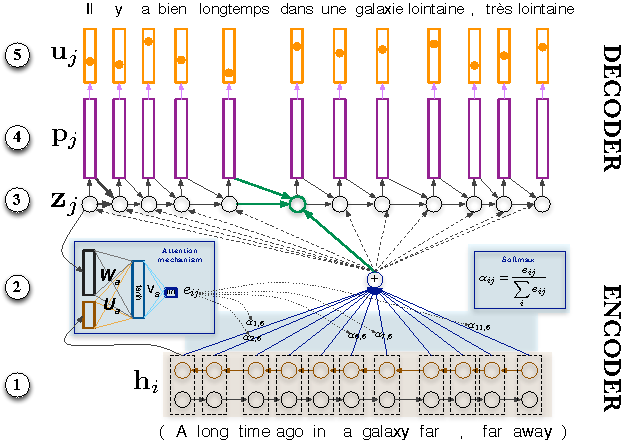
From the diagram above, hi and zj represent all hidden states of encoder and hidden state immediately before the timestep we are in the decoder respectively.The end product of the softmax function gives us the weights which we multiply with all the hidden states from the encoder. A hidden state at a particular timestep with a bigger weight value means more attention is being paid on the word at that timestep. You may have noticed we performed a reduce_sum to produce the context vector. After multiplying each hidden_state with its corresponding weight, we combine all resultant values through a summation. That's it for the attention layer. It returns the context vector and the attention weights.
class Decoder(keras.models.Model):
    def __init__(self, vocab_size, dec_dim=256, embedding_dim=256):
        super(Decoder, self).__init__()

        self.attn = BahdanauAttention(dec_dim)
        self.embedding = keras.layers.Embedding(vocab_size, embedding_dim)
        self.gru = keras.layers.GRU(dec_dim, recurrent_initializer='glorot_uniform',
                                   return_sequences=True, return_state=True)
        self.fc = keras.layers.Dense(vocab_size)

    def call(self, x, hidden, enc_out):
        #x.shape = (16, 1)
        #enc_out.shape = (16, 10, 256)
        #enc_hidden.shape = (16, 256)
        x = self.embedding(x)
        #x.shape = (16, 1, 256)
        context, attn_weights = self.attn(enc_out, hidden)
        #context.shape = (16, 256)
        x = tf.concat((tf.expand_dims(context, 1), x), -1)
        #x.shape = (16, 1, e_c_hidden_size + d_c_embedding_size)
        r_out, hidden = self.gru(x, initial_state=hidden)
        out = tf.reshape(r_out,shape=(-1, r_out.shape[2]))
        # out.shape = (16, 256)
        return self.fc(out), hidden, attn_weights
In the call function, we pass in three parameters, x representing the tensor of a single word, hidden which represents the hidden state of the previous timestep and enc_out which represents all the hidden states of the encoder, we pass x through an embedding layer which maps the single integer token into a dense 256 dimensional vector and concatenate it with the context vector generated by the attention layer. The resultant tensor becomes our input for the Gated Recurrent Network for a single timestep. Finally we pass the output of the GRU through a fully connected layer which outputs a vector of size (batch_size, number of english words). We also return hidden state to be fed into the next timestep and the attention weights for later visualizations. Our complete model is now ready to be trained. Next on the agenda is the training pipeline. We’ll begin with our loss function.
    def loss_fn(real, pred):
        criterion = keras.losses.SparseCategoricalCrossentropy(from_logits=True,
                                                               reduction='none')
        mask = tf.math.logical_not(tf.math.equal(real, 0))
        _loss = criterion(real, pred)
        mask = tf.cast(mask, dtype=_loss.dtype)
        _loss *= mask
        return tf.reduce_mean(_loss)
We use keras’s sparse categorical cross entropy module since we have a large number of categories(number of english words). We create a mask that asserts that the padding tokens are not included in calculating the loss.Now let’s dive in into our training pipeline.
def train_step(input_tensor, target_tensor, enc_hidden):
    optimizer = tf.keras.optimizer.Adam()
    loss = 0.0
    with tf.GradientTape() as tape:

        batch_size = input_tensor.shape[0]
        enc_output, enc_hidden = encoder(input_tensor, enc_hidden)

        SOS_tensor = np.array([SOS_token])
        dec_input = tf.squeeze(tf.expand_dims([SOS_tensor]*batch_size, 1), -1)
        dec_hidden = enc_hidden

        for tx in range(target_tensor.shape[1]-1):
            dec_out, dec_hidden, _ = decoder(dec_input, dec_hidden,
                                            enc_output)
            loss += loss_fn(target_tensor[:, tx], dec_out)
            dec_input = tf.expand_dims(target_tensor[:, tx], 1)

    batch_loss = loss / target_tensor.shape[1]
    t_variables = encoder.trainable_variables + decoder.trainable_variables
    gradients = tape.gradient(loss, t_variables)
    optimizer.apply_gradients(zip(gradients, t_variables))
    return batch_loss
The above snippet implements a single training step. In our single training step, we pass the input_tensor which represent the input sentence through the forward propagation pipeline of the Encoder. This return the enc_output(hidden_state of all timesteps) and enc_hidden(last hidden_state). Notice that the last hidden_state of the encoder is used as the initial hidden_state of the decoder. In the decoding part, we use a technique called teacher forcing where instead of using the predicted word as input for the next timestep, we use the actual word. At the start of decoding, we feed the Start Of Sentence token as input and maximize the probability of the decoder predicting the first word in the output sequence as it output. We then take the actual first word and feed it into the second timestep and maximize the probability of the decoder predicting the second word in the output sequence as it output. This continues sequentially until we reach the End of Sentence token<EOS>. We accumulate all the losses, derive the gradients and train both networks end-to-end with the gradients. That’s all it takes to complete a single training step. Let’s implement a helper function to save our model at certain points during our training.
def checkpoint(model, name=None):
    if name is not None:
        model.save_weights('/content/gdrive/My Drive/{}.h5'.format(name))
    else:
        raise NotImplementedError
The final part of our training pipeline is a training loop. It’s pretty simple to understand. All we do is to run through some epochs and at each epoch, we iterate through our dataset and call the train_step function on each batch of the dataset. There are some if-else statements just to log our training statistics on screen. Let’s see how.
EPOCHS = 10
log_every = 50
steps_per_epoch = len(pairs) // BATCH_SIZE

for e in range(1, EPOCHS):

    total_loss = 0.0
    enc_hidden = encoder.init_hidden()

    for idx, (input_tensor, target_tensor) in enumerate(dataset.take(steps_per_epoch)):
        batch_loss = train_step(input_tensor, target_tensor, hidden)
        total_loss += batch_loss

        if idx % log_every == 0:
            print("Epochs: {} batch_loss: {:.4f}".format(e, batch_loss))
            checkpoint(encoder, 'encoder')
            checkpoint(decoder, 'decoder')

    if e % 2 == 0:
        print("Epochs: {}/{} total_loss: {:.4f}".format(
        e, EPOCHS, total_loss / steps_per_epoch))
Running this snippet trains our model. This might take some time if you intend to train the model on your local machine’s CPU. I suggest you use Google Colab or Kaggle kernels or more preferably Paperspace Gradient notebooks which have GPU-enabled environments to speed-up training. I have already done my training so I’m going to load my model’s weights and demonstrate to you how good a model we’ve built.
encoder.load_weights('/content/gdrive/My Drive/encoder.h5')
decoder.load_weights('/content/gdrive/My Drive/decoder.h5')
In order to perform the translation, we need to write a function much like what we did in the train_step function but instead of feeding in the actual word at a particular time step into the next time step, we feed in the word predicted by our network. This algorithm is known as Greedy search.

Let’s dive into the code as see what’s happening.
def translate(sentence, max_length=10):
    result = ''
    attention_plot = np.zeros((10,10))
    sentence = normalizeString(sentence)
    sentence = sentencetoIndexes(sentence, input_lang)
    sentence = keras.preprocessing.sequence.pad_sequences([sentence],padding='post',
                                                      maxlen=max_length, truncating='post')

    encoder_hidden = hidden = [tf.zeros((1, 256))]

    enc_out, enc_hidden = encoder(sentence, encoder_hidden)

    dec_hidden = enc_hidden
    SOS_tensor = np.array([SOS_token])
    dec_input = tf.squeeze(tf.expand_dims([SOS_tensor], 1), -1)

    for tx in range(max_length):
        dec_out, dec_hidden, attn_weights = decoder(dec_input,
                                                   dec_hidden, enc_out)
        attn_weights = tf.reshape(attn_weights, (-1, ))
        attention_plot[tx] = attn_weights.numpy()
        pred = tf.argmax(dec_out, axis=1).numpy()
        result += output_lang.int2word[pred[0]] + " "
        if output_lang.int2word[pred[0]] == "EOS":
            break
        dec_input = tf.expand_dims(pred, axis=1)
    return result, attention_plot
Our translate function takes in two parameters, the sentence and maximum length for the input sentence . The sentence passes through a preprocessing stage where it is normalized, converted to integer values and padded. The preprocessed tensor is passed through the encoder to generate the encoder_output and encoder_hidden which are conveyed to the decoder. Notice that at the decoding stage, the decoder first receives the Start of Sentence<SOS> token as the first input word or token. After propagating the Start of Sentence token forward through the first time step along with the encoder last hidden state and all the hidden states of the encoder for attention mechanism, a probability distribution is outputted with the word intended to be predicted having the highest value in the distribution. Taking the argmax of this distribution just returns the integer position of the intended word (maximum value in the distribution) in the distribution. This integer position is actually the integer correspondent of the word in the int2word mapping in our Language class. We retrieve the string word using the int2word dictionary, append it to a string and feed back the integer correspondent into the next time step and repeat the process until we encounter the End of Sentence token. We also populate our attention_plot data container with the attention weights produced at each timestep. The final string returned should have the translation for the input sentence we entered. Let’s see a demo!


It works with charm. Let’s also look at some wrong predictions the network make. Admittedly, I really had a hard time searching for sentences for the network to make wrong predictions.

The correct prediction according to Google Translate is : I am older than you.

Correct translation: I don’t like the way you are talking to me.
Let’s wrap this article up by verifying that our attention mechanism is working properly. We are going to visualize how much attention the network is paying to each word in the input sentence when generating a word in the output sentence.
    def plot_attention(attention, sentence, predicted_sentence):
        fig = plt.figure(figsize=(10,10))
        ax = fig.add_subplot(1, 1, 1)
        ax.matshow(attention, cmap='viridis')

        fontdict = {'fontsize': 14}

        ax.set_xticklabels([''] + sentence, fontdict=fontdict, rotation=90)
        ax.set_yticklabels([''] + predicted_sentence, fontdict=fontdict)

        ax.xaxis.set_major_locator(ticker.MultipleLocator(1))
        ax.yaxis.set_major_locator(ticker.MultipleLocator(1))

        plt.show()

Not that perfect when compared to the plot shown in the attention mechanism paper but we can see that it's doing a pretty awesome job with some words like"il" and"he" as well as"eglise" and"church".
Next steps
So that's it for this tutorial. As a next step, I urge you use a much larger dataset such as WMT-17. This can be easily obtained from the TensorFlow-datasets framework.
Also, the knowledge you gained here can be extended to other domains such as chat-bots and image captioning. Don't stop here. Keep digging.
The field of machine translation and sequence to sequence models is an area with much attention from the research community and hence novel models are constantly being developed. One of these state of the art models recently developed is the Transformer network which can also perform translation tasks certainly better than the architecture we just built. I think you should check out that also.
Jupyter Notebook
Acknowledgement
A big thank you to the TensorFlow team for a well documented webpage about the topic discussed. I really got inspired by the work.
About me
I am an undergraduate student currently studying Electrical and Electronic Engineering. I am also a deep learning enthusiast and writer. My work mostly focuses on computer vision and natural language processing. I'm hoping to one day break into the field of autonomous vehicles.You can follow along on twitter(@henryansah083): https://twitter.com/henryansah083?s=09 LinkedIn: https://www.linkedin.com/in/henry-ansah-6a8b84167/.