Building Your First NLP Application to Detect SPAM

The "first" step is always the hardest. There are two possible aspects attached—it shouldn’t be too complicated to discourage further exploration and shouldn’t be too easy not to be able to comprehend the abstract intricacies.

Natural Language Processing (NLP) is a collection of a wide range of concepts. While it can be challenging to choose a starting point, in this tutorial we’ll cover the prerequisites required to build a simple NLP application, and later move on to building one.

Here’s what we'll be covering:

• What is Natural Language Processing?
• The Two Primitive Branches—Syntax & Semantics
• Applications of NLP
• The NLP Vocabulary
• Coding a Simple NLP Application

Without any further ado, let’s get started!

What is Natural Language Processing?

One way humans comprehend the universe is through language. Language is mostly verbal or written, although something like a gesture is also considered language. Language can also be articulated through minor factors like word choice, tone, formality, and a million other variables.

Imagine how challenging it would be as a human to analyze a vast corpus of sentences in multiple languages. Is the task feasible? Your comprehension would be limited. It would be difficult to establish a relation between words and concepts – yet you still might be surprised by how much you do understand.

What if we have a machine to implement tasks that deal with natural language instead? A machine doesn’t possess the intelligence to run such tasks without training, but if we plug in the problem, required information, and algorithms, we can make the machine think cognitively.

Here comes NLP, or natural language processing. The goal of NLP is to enable a machine to make sense of human language. NLP contains subfields like speech recognition and natural language understanding and in general, makes use of various algorithms to convert the human language to a series of syntactic or semantic representations.

The Two Primitive Branches

NLP primarily depends on two essential sub-tasks: syntax and semantics.

Syntax

Syntax pertains to rules which govern the arrangement of words in a sentence. In NLP, a set of grammatical rules are used to govern the syntax of the text.

Let’s consider the following two sentences:

1. I am reading a book.
2. Reading a book I am.

Both sentences have the same set of words, but it's clear to any English speaker that the first sentence is syntactically correct, while the second is not. We know this because we've learned explicitly or implicitly that the second option is bad grammar.

A computer doesn't have this kind of grammatical knowledge. We’d have to train it to learn the distinction.

These are concepts that NLP utilizes to distinguish sentences:

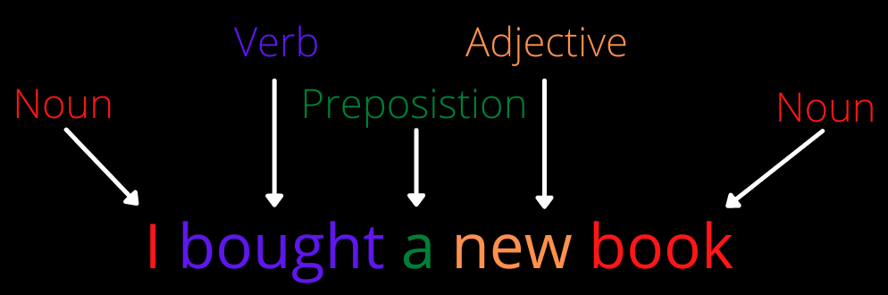
1. Label every word with its appropriate speech. This process is called Part-of-speech (PoS) tagging. For example, in the sentence “I am reading a book,” “I” is a pronoun, “am” and “reading” are verbs, “a” is a determiner, and “book” is a noun. There could be cases where a word could have one PoS in one sentence and a different PoS in the other; the word “watch” in the sentence “my watch had stopped” is a noun, and in the sentence “Lucy watched him go” is a verb. NLP has to have the intelligence to associate the right PoS with every word.

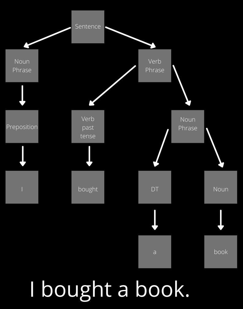
2. Segregate the sentence into its appropriate grammatical constituents. This process is called Constituency Parsing. For example, in the sentence “She enjoys playing tennis,” “She” is a noun phrase (NP), and “enjoys playing tennis” is a verb phrase (VP). Constituency parsing helps in establishing a relation between phrases in a sentence.

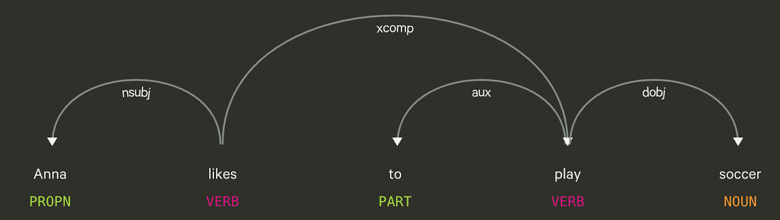
3. Establish a dependency between any two words in a sentence. This process is called Dependency Parsing. Unlike constituency parsing, dependency parsing establishes a relation between the words. For example, consider the sentence “Anna likes to play soccer.” The figure above shows the dependency graph generated using Explosion’s dependency parser.

Relevant terminology:

• nsubj is a nominal subject which is a noun phrase and is the syntactic subject of a clause.
• xcomp is an open clausal complement of a verb or an adjective which is a predicative or clausal complement without its own subject.
• aux is an auxiliary of a clause which is a non-main verb of the clause.
• dobj is a direct object of a verb phrase. It is the noun phrase that is the (accusative) object of the verb.

To learn more about dependency relations, I recommend checking out the Stanford typed dependencies manual.

Depending on the language and text at hand, the appropriate syntax parsing techniques are used.

Semantics

Semantics is the meaning of a text. In NLP, semantic analysis refers to the extraction and interpretation of meaning from the text.

Lexical semantics is a crucial concept in semantic analysis. The following are some of the key elements within the study of lexical semantics to understand:

1. Hyponyms: a word of more specific meaning than a general word e.g. black is a hyponym of color
2. Homonym: two words with the same spelling or pronunciation with different meanings e.g. right, as in the opposite of left, and right, as in correct
3. Meronym: when a part of something is used to refer to the whole e.g. sails on the water refer to ships on the water
4. Polysemy: many possible meanings for a word e.g. sound is a polysemy with multiple meanings
5. Synonym: a word that has the same meaning as another word e.g. bold and audacious are synonyms
6. Antonyms: a word that has the opposite meaning as another word e.g. true and false are antonyms

Vaguely, these are utilized by NLP to check the meaningfulness of text. Moreover, NLP checks for semiotics and collocations. Both syntax and semantics taken together help NLP understand the text’s intricacies.

Applications of NLP

Applications for NLP abound. Some of the most popular include:

• Speech recognition
• Automatic summarization
• Chatbots
• Question answering models
• Text classification
• Sentiment analysis
• Language translator
• Search autocomplete
• Text autocorrect

The NLP Vocabulary

Language in itself is complex, and NLP follows in the same footsteps. It has a collection of concepts to tackle the complexity of language.

Corpus

A corpus is a collection of text documents.

Lexicon

A lexicon is a vocabulary of a language. For example, in football/soccer, “offsides,” “half-volley,” and “penalty kick” are all part of the sport's lexicon.

Tokenization

Tokenization is the process of splitting text into words (or) tokens. For example, consider the sentence “Washington D.C. is the capital city of the United States.” The tokens would then be Washington, D.C., is, the, capital, city, of, the, United, and States.

And if we do not want to split up Washington and D.C.? We first have to identify the named entities and, later, tokenize our text. (refer to n-grams section below)

Thus, tokenization is more than splitting up the text using white space.

Parsing

Parsing encapsulates syntactic and semantic analysis phases. Parsing, in general, is breaking text into its respective constituents based on a specific agenda. For example, syntactic parsing breaks text into its syntactic components, which could be based on PoS, constituency, or dependency parsing. Semantic parsing is the task of converting natural language utterances into formal meaning representations [ref].

Parsing usually generates a parsed tree which provides a visual representation of the parsed output.

Normalization

Text normalization is the conversion of text to its standard form. Here are its two variants:

Stemming

Stemming is reducing the words to their stem – usually by removing the suffixes. For example, consider the word “crammed”. When the suffix “med” is removed, we get the word “cram”, which is the stem.

Stemming is a data pre-processing technique that helps in simplifying the process of understanding the text, with which we wouldn’t have a huge database!

There are two kinds of errors that could pop up during stemming:

• Over-stemming: When two words are stemmed to the same stem (or root word), which actually belong to two different stems. For example, consider the words universal, university, and universe [ref]. These words are stemmed to “univers” although they belong to different domains in the natural language.
• Under-stemming: When two words are stemmed to a different stem (or root word) that do not belong to different stems. For example, consider the words, data, and datum. These words are stemmed to “data” and “datum” respectively, although they belong to the same domain.

Examples of stemming algorithms include Porter’s algorithm, Lovins Stemmer, Dawson Stemmer, etc.

Lemmatization

The other variant of normalization is called lemmatization and it refers to mapping a word to its root dictionary form, which is called a “lemma.” This could seem similar to the stemming approach, however, it uses a different technique to derive the lemma. For example, the lemma for the words “are, am, is” is “be” (given the PoS as a verb).

Lemmatization is a much more resource-intensive task than stemming as it requires more knowledge about the text’s structure.

Stop Word Removal

Stop words are commonly occurring words such as articles, pronouns, and prepositions. The removal process excludes the unnecessary words of little value and helps us focus more on the text that requires our attention.

The best part is that it reduces dependency on a vast database, consumes less time in analyzing the text, and helps improve the performance.

However, this isn’t a mandatory NLP technique that has to be applied in every algorithm. In applications such as text summarization, sentiment analysis, and language translation, removal of stop words isn’t advisable due to the loss of necessary information.

Consider a scenario where the word “like” is removed. In an application such as sentiment analysis, this removal could wipe out the positivity exuded by the text.

Bag of Words (BoW)

As the name indicates, a bag of words counts the occurrences of words in the text, disregarding the order of words and the structure of the document.

For example, consider the following two lines of text:

Your problems are similar to mine
Your idea seems to be similar to mine

First, let’s make a list of all the occurring words:

1. your
2. problems
3. are
4. similar
5. to
6. mine
7. idea
8. seems
9. be

BoW creates vectors (in our case, let’s consider a binary vector) as follows:

1. Your problems are similar to mine – [1, 1, 1, 1, 1, 1, 0, 0, 0]
2. Your idea seems to be similar to mine – [1, 0, 0, 1, 1, 1, 1, 1, 1]

As can be inferred, the ordering of words is discarded. Moreover, it does not scale to larger vocabularies. This can be resolved using n-grams and word embeddings (refer to the following sections).

The bag of words approach could pose a problem wherein the stop words are assigned a greater frequency than the informational words. Term Frequency-Inverse Document Frequency (TF-IDF) helps in rescaling the frequency of words by how often they appear in the texts so that stop words could get penalized. The TF-IDF technique rewards the frequently occurring words but punishes the too commonly occurring words in several texts.

The bag of words approach (with or without TF-IDF) might not be the best approach towards understanding the meaning of the text however it’s helpful in an application like text classification.

N-Grams

An n-gram is a sequence of n words. Consider the sentence “n-gram is a contiguous sequence of n items.” If n is set to 2 (so-called bigrams), the n-grams would be:

• n-gram is
• is a
• a contiguous
• contiguous sequence
• sequence of
• of n
• n items

N-grams are used for auto-completion of sentences, text summarization, auto spell check, etc.

N-grams could be more informative than BoW because they capture the context around each word (which depends on the value of n).

Word Embeddings

Word embeddings help in representing individual words as real-valued vectors in the lower dimensional space. Put simply, it’s the conversion of text to numerical data (vectors) which can facilitate the analysis by an NLP model.

BoW vs. Word Embeddings

Unlike BoW, word embeddings use a predefined vector space to map words irrespective of corpus size. Word embeddings can determine the semantic relationship between words in the text, whereas BoW cannot.

In general, BoW is useful if:

• Your dataset is small
• Language is domain-specific

Examples of off-the-shelf word embedding models include Word2Vec, GloVe, and fastText.

Named Entity Recognition (NER)

NER categorizes informative words (so-called “named entities”) into various categories: place, time, person, etc. Some notable applications of NER include search and recommendation engines, categorizing user complaints and requests, text classification, etc.

You can use spaCy or NLTK to perform NER on your corpus.

Coding a Simple NLP Application

In this example, we will detect spam messages by first pre-processing the text corpus comprising spam and non-spam messages using the Bag of Words (BoW) approach. Later, we will train a model on the processed messages using an XGBoost model.

Here’s a step-by-step process that walks you through the data pre-processing and modeling process.

Step 1: Import the Libraries

First, let’s install and import the necessary libraries.

# You may need to install libraries
! pip install pandas
! pip install nltk
! pip install scikit-learn

# Import libraries
import string
import nltk
import pandas as pd
from nltk.corpus import stopwords
from sklearn import metrics
from sklearn.feature_extraction.text import CountVectorizer
from sklearn.model_selection import train_test_split

nltk (Natural Language ToolKit) is the primary package that helps us in NLP-ing our data.

scikit-learn is helpful to build, train, and test the efficacy of the model.

Step 2: Preprocess the Dataset

Preprocessing is the process of cleaning up the data. First, we fetch the data and comprehend its structure. As you can see below, our text for each message is held in the v2 column, and the classification target in v1. If a text is spam, it is marked in v1 as "spam", and if not, it is marked as "ham."

# Read the dataset
messages = pd.read_csv(
    "spam.csv", encoding="latin-1",
    index_col=[0]
)
messages.head()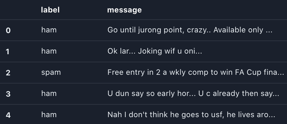

Next, we define a text_preprocess method that removes punctuations, stop-words, and non-alphabets.

def text_preprocess(message):
    # Remove punctuations
    nopunc = [char for char in message if char not in string.punctuation]

    # Join the characters again
    nopunc = "".join(nopunc)
    nopunc = nopunc.lower()

    # Remove any stopwords and non-alphabetic characters
    nostop = [
        word
        for word in nopunc.split()
        if word.lower() not in stopwords.words("english") and word.isalpha()
    ]

    return nostop

Let's see how many spam and ham (non-spam) messages constitute our dataset.

spam_messages = messages[messages["label"] == "spam"]["message"]
ham_messages = messages[messages["label"] == "ham"]["message"]
print(f"Number of spam messages: {len(spam_messages)}")
print(f"Number of ham messages: {len(ham_messages)}")

# Output
Number of spam messages: 747
Number of ham messages: 4825

Next, we check the top ten words that repeat the most in both ham and spam messages.

# Download stopwords
nltk.download('stopwords')

# Words in spam messages
spam_words = []
for each_message in spam_messages:
    spam_words += text_preprocess(each_message)
    
print(f"Top 10 spam words are:\n {pd.Series(spam_words).value_counts().head(10)}")

# Output
Top 10 spam words are:
call      347
free      216
txt       150
u         147
ur        144
mobile    123
text      120
claim     113
stop      113
reply     101
dtype: int64

# Words in ham messages
ham_words = []
for each_message in ham_messages:
    ham_words += text_preprocess(each_message)
    
print(f"Top 10 ham words are:\n {pd.Series(ham_words).value_counts().head(10)}")

# Output
Top 10 ham words are:
u       972
im      449
get     303
ltgt    276
ok      272
dont    257
go      247
ur      240
ill     236
know    232
dtype: int64

This information isn't needed to conduct our modeling; however, it is critical to perform exploratory data analysis to help inform our model.

Here comes the crucial step: we text_preprocess our messages.

# Remove punctuations/stopwords from all messages
messages["message"] = messages["message"].apply(text_preprocess)
messages.head()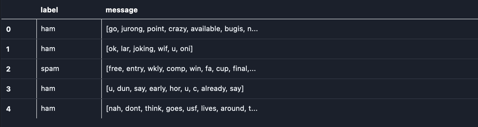

The output produced will be a list of tokens. A string can be understood by a model, not a list of tokens. Hence, we convert the list of tokens to a string.

# Convert messages (as lists of string tokens) to strings
messages["message"] = messages["message"].agg(lambda x: " ".join(map(str, x)))
messages.head()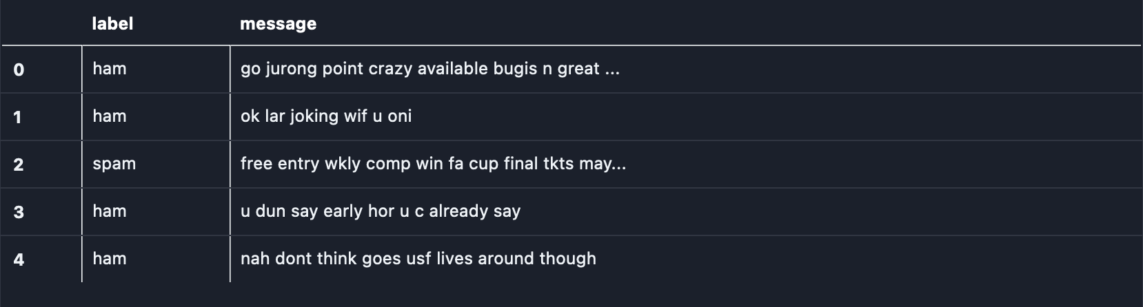

Step 3: The Bag of Words Approach

The CountVectorizer() class in the scikit-learn library is useful in defining the BoW approach. We first fit the vectorizer to the messages to fetch the whole vocabulary.

# Initialize count vectorizer
vectorizer = CountVectorizer()
bow_transformer = vectorizer.fit(messages["message"])

# Fetch the vocabulary set
print(f"20 BOW Features: {vectorizer.get_feature_names()[20:40]}")
print(f"Total number of vocab words: {len(vectorizer.vocabulary_)}")

# Output
20 BOW Features: ['absence', 'absolutely', 'abstract', 'abt', 'abta', 'aburo', 'abuse', 'abusers', 'ac', 'academic', 'acc', 'accent', 'accenture', 'accept', 'access', 'accessible', 'accidant', 'accident', 'accidentally', 'accommodation']
Total number of vocab words: 8084

As can be inferred, there are about 8084 words in the text corpus we fetched.

We transform the string messages to numerical vectors to simplify the model-building and training process.

# Convert strings to vectors using BoW
messages_bow = bow_transformer.transform(messages["message"])

# Print the shape of the sparse matrix and count the number of non-zero occurrences
print(f"Shape of sparse matrix: {messages_bow.shape}")
print(f"Amount of non-zero occurrences: {messages_bow.nnz}")

# Output
Shape of sparse matrix: (5572, 8084)
Amount of non-zero occurrences: 44211

BoW builds a sparse matrix mapping the occurrence of every word to the corpus vocabulary. Thus, this approach leads to building a sparse matrix, or a matrix that is mostly comprised of zeros. This format allows for the conversion of the text into an interpretable encoding of linguistic information that a model can make use of.

Step 4: The TF-IDF Approach

In the Bag of Words (BoW) section, we learned how BoW’s technique could be enhanced when combined with TF-IDF. Here, we run our BoW vectors through TF-IDF.

# TF-IDF
from sklearn.feature_extraction.text import TfidfTransformer

tfidf_transformer = TfidfTransformer().fit(messages_bow)

# Transform entire BoW into tf-idf corpus
messages_tfidf = tfidf_transformer.transform(messages_bow)
print(messages_tfidf.shape)

# Output
(5572, 8084)

Step 5: Build the XGBoost Model

XGBoost is a gradient boosting technique that can do both regression and classification. In this case, we will be using an XGBClassifier to classify our text as either "ham" or "spam".

First, we convert the “spam” and “ham” labels to 0 and 1 (or vice-versa) as XGBoost accepts only numerics.

# Convert spam and ham labels to 0 and 1 (or, vice-versa)
FactorResult = pd.factorize(messages["label"])
messages["label"] = FactorResult[0]
messages.head()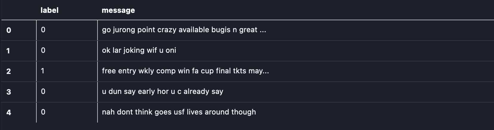

Next, we split the data to train and test datasets.

# Split the dataset to train and test sets
msg_train, msg_test, label_train, label_test = train_test_split(
    messages_tfidf, messages["label"], test_size=0.2
)

print(f"train dataset features size: {msg_train.shape}")
print(f"train dataset label size: {label_train.shape}")

print(f"test dataset features size: {msg_test.shape}")
print(f"test dataset label size: {label_test.shape}")

# Output
train dataset features size: (4457, 8084)
train dataset label size: (4457,)
test dataset features size: (1115, 8084)
test dataset label size: (1115,)

To train the model, we first install the XGBoost library.

# Install xgboost library
! pip install xgboost

We train the classifier.

# Train an xgboost classifier
from xgboost import XGBClassifier

# Instantiate our model
clf = XGBClassifier()

# Fit the model to the training data
clf.fit(msg_train, label_train)

Next, we make predictions on the training dataset.

# Make predictions
predict_train = clf.predict(msg_train)

print(
    f"Accuracy of Train dataset: {metrics.accuracy_score(label_train, predict_train):0.3f}"
)

# Output
Accuracy of Train dataset: 0.989

To get an essence of how our model fared, let’s do an example prediction.

# an example prediction
print(
    "predicted:",
    clf.predict(
        tfidf_transformer.transform(bow_transformer.transform([messages["message"][9]]))
    )[0],
)
print("expected:", messages["label"][9])

# Output
predicted: 1
expected: 1

And yes, it worked!

Finally, we find the overall accuracy of the model on the test data.

# print the overall accuracy of the model
label_predictions = clf.predict(msg_test)
print(f"Accuracy of the model: {metrics.accuracy_score(label_test, label_predictions):0.3f}")

# Output
Accuracy of the model: 0.975

Conclusion

You’ve taken your first step into a larger world! NLP is a prominent topic that gained significance over the years owing to the ease of handling large amounts of natural language data. You’re now prepped to handle the more profound NLP concepts.

I hope you enjoyed reading this article!

References

1. https://www.kaggle.com/dktalaicha/sms-spam-detection-with-nlp
2. https://towardsdatascience.com/your-guide-to-natural-language-processing-nlp-48ea2511f6e1
3. https://monkeylearn.com/blog/semantic-analysis/