Writing CNNs from Scratch in PyTorch

Introduction

In this article, we will be building Convolutional Neural Networks (CNNs) from scratch in PyTorch, and seeing them in action as we train and test them on a real-world dataset.

We will start by exploring what CNNs are and how they work. We will then look into PyTorch and start by loading the CIFAR10 dataset using torchvision (a library containing various datasets and helper functions related to computer vision). We will then build and train our CNN from scratch. Finally, we will test our model.

Below is the outline of the article:

• Introduction
• Convolutional Neural Networks
• PyTorch
• Data Loading
• CNN from Scratch
• Setting Hyperparameters
• Training
• Testing

Convolutional Neural Networks

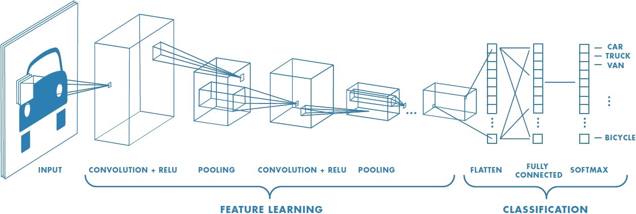
A convolutional neural network (CNN) takes an input image and classifies it into any of the output classes. Each image passes through a series of different layers – primarily convolutional layers, pooling layers, and fully connected layers. The below picture summarizes what an image passes through in a CNN:

Convolutional Layer

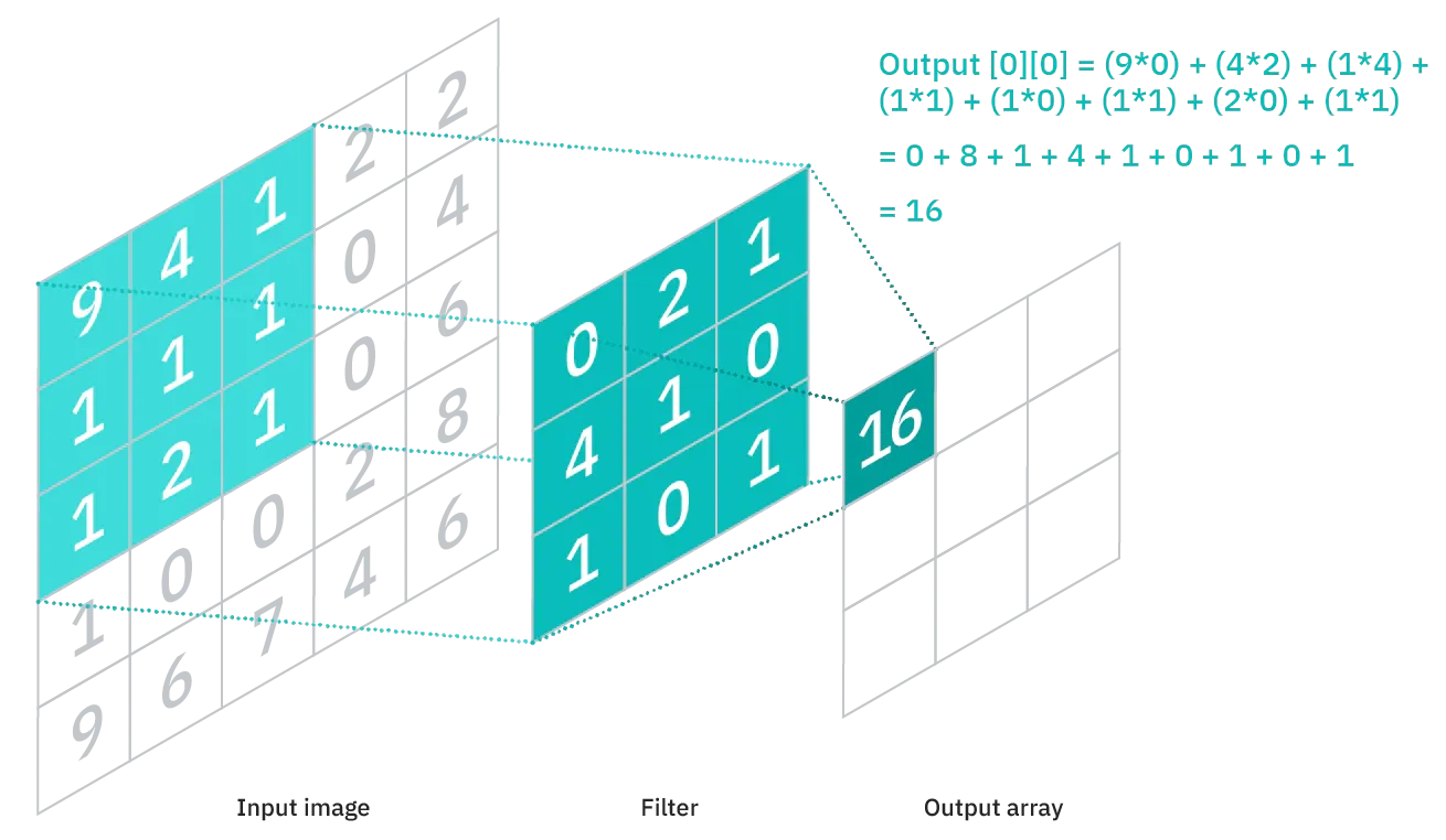
The convolutional layer is used to extract features from the input image. It is a mathematical operation between the input image and the kernel (filter). The filter is passed through the image and the output is calculated as follows:

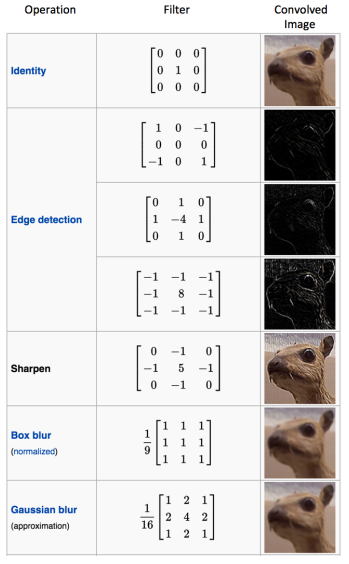
Different filters are used to extract different kinds of features. Some common features are given below:

Pooling Layers

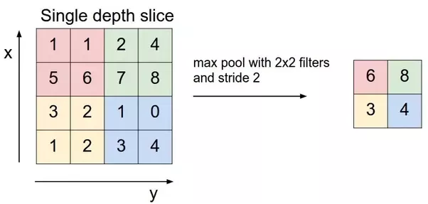
Pooling layers are used to reduce the size of any image while maintaining the most important features. The most common types of pooling layers used are max and average pooling which take the max and the average value respectively from the given size of the filter (i.e, 2x2, 3x3, and so on).

Max pooling, for example, would work as follows:

PyTorch

PyTorch is one of the most popular and widely used deep learning libraries – especially within academic research. It's an open-source machine learning framework that accelerates the path from research prototyping to production deployment and we'll be using it today in this article to create our first CNN.

Data Loading

Dataset

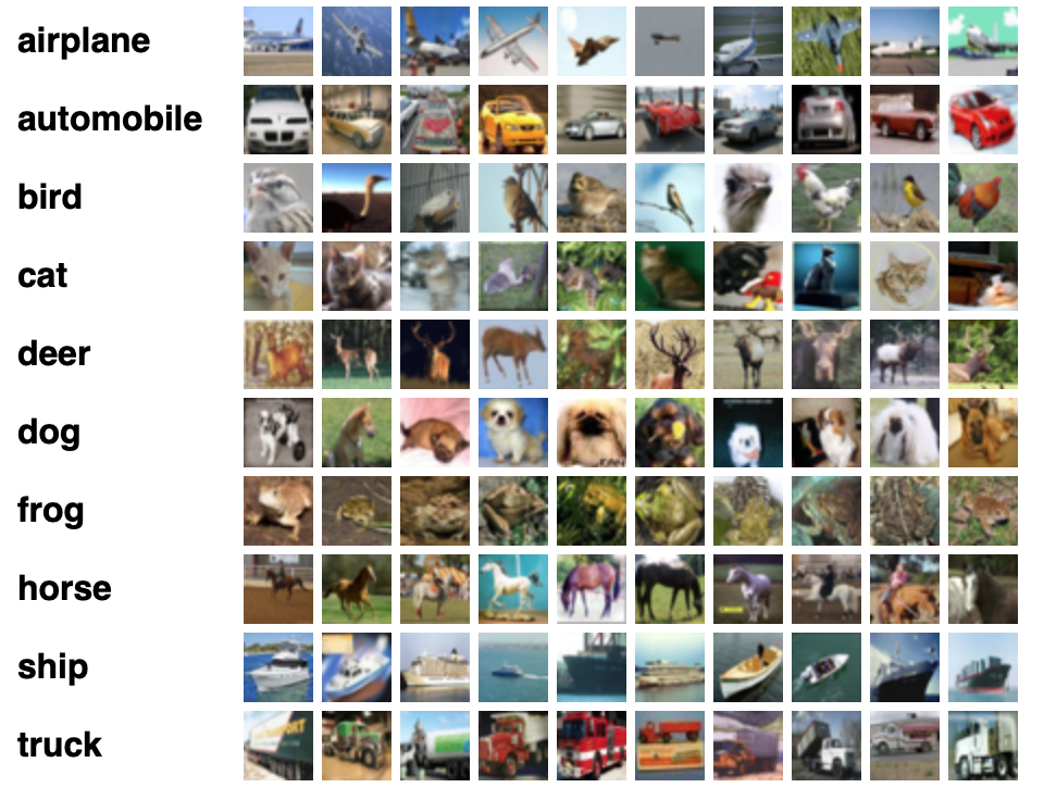
Let's start by loading some data. We will be using the CIFAR-10 dataset. The dataset has 60,000 color images (RGB) at 32px x 32px belonging to 10 different classes (6000 images/class). The dataset is divided into 50,000 training and 10,000 testing images.

You can see a sample of the dataset along with their classes below:

Importing the Libraries

Let's start by importing the required libraries and defining some variables:

# Load in relevant libraries, and alias where appropriate
import torch
import torch.nn as nn
import torchvision
import torchvision.transforms as transforms

# Define relevant variables for the ML task
batch_size = 64
num_classes = 10
learning_rate = 0.001
num_epochs = 20

# Device will determine whether to run the training on GPU or CPU.
device = torch.device('cuda' if torch.cuda.is_available() else 'cpu')

device will determine whether to run the training on GPU or CPU.

Dataset Loading

To load the dataset, we will be using the built-in datasets in torchvision. It provides us with the ability to download the dataset and also apply any transformations we want.

Let's look at the code first:

# Use transforms.compose method to reformat images for modeling,
# and save to variable all_transforms for later use
all_transforms = transforms.Compose([transforms.Resize((32,32)),
                                     transforms.ToTensor(),
                                     transforms.Normalize(mean=[0.4914, 0.4822, 0.4465],
                                                          std=[0.2023, 0.1994, 0.2010])
                                     ])
# Create Training dataset
train_dataset = torchvision.datasets.CIFAR10(root = './data',
                                             train = True,
                                             transform = all_transforms,
                                             download = True)

# Create Testing dataset
test_dataset = torchvision.datasets.CIFAR10(root = './data',
                                            train = False,
                                            transform = all_transforms,
                                            download=True)

# Instantiate loader objects to facilitate processing
train_loader = torch.utils.data.DataLoader(dataset = train_dataset,
                                           batch_size = batch_size,
                                           shuffle = True)


test_loader = torch.utils.data.DataLoader(dataset = test_dataset,
                                           batch_size = batch_size,
                                           shuffle = True)

Let's dissect this piece of code:

• We start by writing some transformations. We resize the images, convert them to tensors and normalize them by using the mean and standard deviation of each band in the input images. You can calculate these as well, but they are available online.
• Then, we load the dataset: both training and testing. We set download equal to True so that it is downloaded if not already downloaded.
• Loading the whole dataset into the RAM at once is not a good practice and can seriously halt your computer. That's why we use data loaders, which allow you to iterate through the dataset by loading the data in batches.
• We then create two data loaders (for train/test) and set the batch size, along with shuffle, equal to True, so that images from each class are included in a batch.

CNN from Scratch

Before diving into the code, let's explain how you define a neural network in PyTorch.

• You start by creating a new class that extends the nn.Module class from PyTorch. This is needed when we are creating a neural network as it provides us with a bunch of useful methods
• We then have to define the layers in our neural network. This is done in the __init__ method of the class. We simply name our layers, and then assign them to the appropriate layer that we want; e.g., convolutional layer, pooling layer, fully connected layer, etc.
• The final thing to do is define a forward method in our class. The purpose of this method is to define the order in which the input data passes through the various layers

Now, let's dive into the code:

# Creating a CNN class
class ConvNeuralNet(nn.Module):
	#  Determine what layers and their order in CNN object 
    def __init__(self, num_classes):
        super(ConvNeuralNet, self).__init__()
        self.conv_layer1 = nn.Conv2d(in_channels=3, out_channels=32, kernel_size=3)
        self.conv_layer2 = nn.Conv2d(in_channels=32, out_channels=32, kernel_size=3)
        self.max_pool1 = nn.MaxPool2d(kernel_size = 2, stride = 2)
        
        self.conv_layer3 = nn.Conv2d(in_channels=32, out_channels=64, kernel_size=3)
        self.conv_layer4 = nn.Conv2d(in_channels=64, out_channels=64, kernel_size=3)
        self.max_pool2 = nn.MaxPool2d(kernel_size = 2, stride = 2)
        
        self.fc1 = nn.Linear(1600, 128)
        self.relu1 = nn.ReLU()
        self.fc2 = nn.Linear(128, num_classes)
    
    # Progresses data across layers    
    def forward(self, x):
        out = self.conv_layer1(x)
        out = self.conv_layer2(out)
        out = self.max_pool1(out)
        
        out = self.conv_layer3(out)
        out = self.conv_layer4(out)
        out = self.max_pool2(out)
                
        out = out.reshape(out.size(0), -1)
        
        out = self.fc1(out)
        out = self.relu1(out)
        out = self.fc2(out)
        return out

As I explained above, we start by creating a class that inherits the nn.Module class, and then we define the layers and their sequence of execution inside __init__ and forward respectively.

Some things to notice here:

• nn.Conv2d is used to define the convolutional layers. We define the channels they receive and how much should they return along with the kernel size. We start from 3 channels, as we are using RGB images
• nn.MaxPool2d is a max-pooling layer that just requires the kernel size and the stride
• nn.Linear is the fully connected layer, and nn.ReLU is the activation function used
• In the forward method, we define the sequence, and, before the fully connected layers, we reshape the output to match the input to a fully connected layer

Setting Hyperparameters

Let's now set some hyperparameters for our training purposes.

model = ConvNeuralNet(num_classes)

# Set Loss function with criterion
criterion = nn.CrossEntropyLoss()

# Set optimizer with optimizer
optimizer = torch.optim.SGD(model.parameters(), lr=learning_rate, weight_decay = 0.005, momentum = 0.9)  

total_step = len(train_loader)

We start by initializing our model with the number of classes. We then choose cross-entropy and SGD (Stochastic Gradient Descent) as our loss function and optimizer respectively. There are different choices for these, but I found these to result in maximum accuracy when experimenting. We also define the variable total_step to make iteration through various batches easier.

Training

Now, let's start training our model:

# We use the pre-defined number of epochs to determine how many iterations to train the network on
for epoch in range(num_epochs):
	#Load in the data in batches using the train_loader object
    for i, (images, labels) in enumerate(train_loader):  
        # Move tensors to the configured device
        images = images.to(device)
        labels = labels.to(device)
        
        # Forward pass
        outputs = model(images)
        loss = criterion(outputs, labels)
        
        # Backward and optimize
        optimizer.zero_grad()
        loss.backward()
        optimizer.step()

    print('Epoch [{}/{}], Loss: {:.4f}'.format(epoch+1, num_epochs, loss.item()))

            
            

This is probably the trickiest part of the code. Let's see what the code does:

• We start by iterating through the number of epochs, and then the batches in our training data
• We convert the images and the labels according to the device we are using, i.e., GPU or CPU
• In the forward pass we make predictions using our model and calculate loss based on those predictions and our actual labels
• Next, we do the backward pass where we actually update our weights to improve our model
• We then set the gradients to zero before every update using optimizer.zero_grad() function
• Then, we calculate the new gradients using the loss.backward() function
• And finally, we update the weights with the optimizer.step() function

We can see the output as follows:

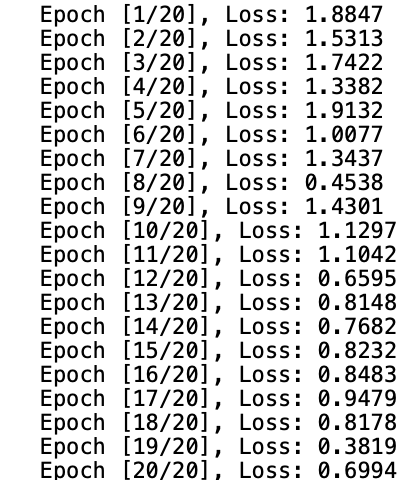
As we can see, the loss is slightly decreasing with more and more epochs. This is a good sign. But you may notice that it is fluctuating at the end, which could mean the model is overfitting or that the batch_size is small. We will have to test to find out what's going on.

Testing

Let's now test our model. The code for testing is not so different from training, with the exception of calculating the gradients as we are not updating any weights:

with torch.no_grad():
    correct = 0
    total = 0
    for images, labels in train_loader:
        images = images.to(device)
        labels = labels.to(device)
        outputs = model(images)
        _, predicted = torch.max(outputs.data, 1)
        total += labels.size(0)
        correct += (predicted == labels).sum().item()
    
    print('Accuracy of the network on the {} train images: {} %'.format(50000, 100 * correct / total))

We wrap the code inside torch.no_grad() as there is no need to calculate any gradients. We then predict each batch using our model and calculate how many it predicts correctly. We get the final result of ~83% accuracy:

And that's it. We managed to create a Convolutional Neural Network from scratch in PyTorch!

Conclusion

We started by learning about CNNs – what kind of layers they have and how they work. We then introduced PyTorch, which is one of the most popular deep learning libraries available today. We learned how PyTorch would make it much easier for us to experiment with a CNN.

Next, we loaded the CIFAR-10 dataset (a popular training dataset containing 60,000 images), and made some transformations on it.

Then, we built a CNN from scratch, and defined some hyperparameters for it. Finally, we trained and tested our model on CIFAR10 and managed to get a decent accuracy on the test set.