Combining Multiple Features and Multiple Outputs Using Keras Functional API

We all wrote our first deep learning code for regression, classification, etc. using public datasets like CIFAR-10, MNIST, or Pima Indians Diabetes.

One common thing we can notice is that the data type of every feature in a given project is the same. Either we will have images to classify or numerical values to input in a regression model.

Have you ever thought about how we can combine data of various types like text, images, and numbers to get not just one output, but multiple outputs like classification and regression?

Real-life problems are not sequential or homogenous in form. You will likely have to incorporate multiple inputs and outputs into your deep learning model in practice.

This article dives deep into building a deep learning model that takes the text and numerical inputs and returns regression and classification outputs.

Overview

• Data Cleaning
• Text Preprocessing
• Magical Model
• Conclusion

Data Cleaning

When we look at a problem with multiple text and numerical inputs and a regression and classification output to be generated, we should first clean our dataset.

For starters, we should avoid data with a lot of Null or NaN valued features. Such values should be replaced with mean, median, etc. such that these records may be used without much effect on overall data.

We can convert numerical values, which are often larger compared to other features, to small values to ensure there is no effect on the weights of the neural network. In order to counter such an effect, one can use techniques such as standardization or min-max scaling to transform the data to a tighter range of values, while still retaining their relationship to one another.

from sklearn.preprocessing import MinMaxScaler

data = [[-1010, 20000], [-50000, 6345], [10000, 1000], [19034, 18200]]

# Instantiate the MinMaxScaler object
scaler = MinMaxScaler()

# Fit it to the data
scaler.fit(data)

# Use transform to output the transformed data
print(scaler.transform(data))

# Output:
[[0.70965032 1.        ]
 [0.         0.28131579]
 [0.86913695 0.        ]
 [1.         0.90526316]]

Text Preprocessing

We can deal with multiple text inputs here in two ways

• Building dedicated LSTMs (Long Short-Term Memory network) for each text feature and later combining the numerical outputs from it
• Combining text features first and then training with a single LSTM

In this article, we will be exploring the second method as it is very effective when handling a huge number of text features with varying lengths.

Combining Text Features

The original dataset has multiple text features that we will have to concatenate. Just adding the strings up wouldn't be efficient. We have to communicate with the model that these are different features in a single string.

The way we deal with this is by joining them with a special “<EOF>” tag between them indicating End of Feature. This doesn't sum any value, but, eventually, LSTM will learn that this tag represents the end of a feature.  Finally, all the text features will be converted to a single input.

"Feature 1 <EOF> Feature 2 <EOF> ….. <EOF> Feature N"

Now we have a single text input and a set of numerical inputs.

Lower casing and Stop words removal

The following techniques are useful during preprocessing.

Lower casing is the process of transforming words to lowercase to provide better clarity. This is helpful in the process of preprocessing and in later stages when we are doing parsing.

Stop words removal is the process of removing commonly used words to focus more on the content of the text feature more. We can use NLTK to remove conventional stop words.

from nltk.corpus import stopwords
stop_words = set(stopwords.words('english'))

# Example sentence 
text = "there is a stranger out there who seems to be the owner of this mansion"

# Split our sentence at each space using .split()
words = text.split()

text = ""

# For each word, if the word isnt in stop words, then add to our new text variable
for word in words:
    if word not in stop_words:
        text += (word+" ")
        
print(text)

Output>> stranger seems owner mansion

Stemming and Lemmatization

These techniques are used to improve semantic analysis.

Stemming means removing prefixes and suffixes from words in order to simplify them. This technique is used to determine domain vocabularies in domain analysis. It helps in reducing variants of a word by converting them to their root form.

As an example, program, programs, and programmer are variants of program.

Here's an example of stemming using NLTK:

from nltk.stem import PorterStemmer  
# Instantiate our stemmer as ps
ps = PorterStemmer()
 
# Example sentence 
sentence = "he is likely to have more likes for the post he posted recently"

# Split our sentence at each space using .split()
words = sentence.split()

sentence = ""

# For each word, get the stem and add to our new sentence variable
for w in words:
    sentence += (ps.stem(w) + " ")
print(sentence)

Output >> he is like to have more like for the post he post recent

Lemmatization is the process of grouping inflected forms of a word. Rather than reducing a word down to its stem, lemmatization instead determines the corresponding dictionary form of the word. This facilitates the model to determine the meaning of a single word.

from nltk.stem import WordNetLemmatizer
lemmatizer = WordNetLemmatizer()

sentence = "It is dangerous to jump to feet on rocky surfaces"
words = sentence.split()
sentence = ""

for word in words:
    sentence+= (lemmatizer.lemmatize(word) + " ")

print(sentence)

Output >> It is dangerous to jump to foot on rocky surface

Train Test Splitting

An important step is to ensure we sample the dataset appropriately and get enough data to test our model after each epoch. Currently, we have two inputs and outputs with text and an array of numerical inputs each. We will split them into train and validation sets for each as given below.

from sklearn.model_selection import train_test_split

y_reg_train, y_reg_val, y_clf_train, y_clf_val, X_text_train, X_text_val, X_num_train, X_num_val = train_test_split(y_reg,y_clf,X_text,X_num,test_size=0.25,random_state=42)

Tokenizing

Before actually doing any NLP modeling, we need numerical values to feed the machine for it to carry out all those mathematical operations. For example, the string “cat” should be converted to a number or a meaningful tensor for the model to process. Tokenizing helps us do this by representing each word with a number.

from keras.preprocessing.text import Tokenizer

# instantiate our tokenizer
tokenizer = Tokenizer(num_words = 10)

# Create a sample list of words to tokenize
text = ["python","is","cool","but","C++","is","the","classic"]

# Fit the Tokenizer to the words
tokenizer.fit_on_texts(text)

# Create a word_index to track tokens
word_index = tokenizer.word_index
print(word_index['python'])

Output >> 2

In our solution, we will have to fit the tokenizer over the training text feature. This is a crucial point in preprocessing, as we should not let the model or tokenizer know about our test inputs if we want to prevent overfitting.

We will store it as a dictionary in word_index. We can save the tokenizer using pickle for future uses like in prediction with just the Model.

Let’s see how we will use tokenizer in our case after fitting it on our corpus.

# Tokenize and sequence training data
X_text_train_sequences = tokenizer.texts_to_sequences(X_text_train)

# Use pad_sequences to transforms a list (of length num_samples) of sequences (lists of integers) into a 2D Numpy array of shape (num_samples, num_timesteps)
X_text_train_padded = pad_sequences(X_text_train_sequences,maxlen=max_length,
                    padding=padding_type, truncating=trunction_type)
                    
# Tokenize and sequence validation data                   
X_text_val_sequences = tokenizer.texts_to_sequences(X_text_val)

# pad_sequences for validation set
X_text_val_padded = pad_sequences(X_text_val_sequences,maxlen=max_length,
                    padding=padding_type, truncating=trunction_type)

Embedding Layer with GloVe

Embeddings give dimensions to each word. Imagine “King” being stored as 102 in our tokenizer. Would that mean anything? We need to express the dimensions of a word and embedding layers help us in that.

It is often better to use pre-trained embedding layers like GloVe to get the most out of our data. Embeddings turn a word_index in tokenizer into a matrix of size (1, N) given N dimensions of the word.

Note: Download GloVe from here.

import numpy as np
# Download glove beforehand

# Here we are using the 100 Dimensional embedding of GloVe  
f = open('glove.6B/glove.6B.100d.txt')   
for line in f:       
   values = line.split()       
   word = values[0]       
   coefs = np.asarray(values[1:], dtype='float32') 
   embeddings_index[word] = coefs   
f.close()

# Creating embedding matrix for each word in Our corpus
embedding_matrix = np.zeros((len(word_index) + 1, 100))   
for word, i in word_index.items():   
   embedding_vector = embeddings_index.get(word)   
   if embedding_vector is not None:   
       # words not found in the embedding index will be all-zeros.  
       embedding_matrix[i] = embedding_vector

Now we have an embedding matrix to input as weights in our embedding layer.

Magical Model

We have done all the preprocessing needed, and now we have our X and Y values to input into a model. We will use Keras Functional API here to build this special model.

Before we jump right into the code it’s important to understand why a sequential model is not enough. A beginner would be familiar with sequential models, as they help us build a linearly flowing model quickly.

from keras.layers import Dense, Embedding, LSTM
from keras.models import Model
from keras.models import Sequential

# Instantiate a sequential NN
model = Sequential([       
  Embedding(len(word_index) + 1,
            100,
            weights=[matrix_embedding],
            input_length=max_length,
            trainable=False)
  LSTM(embedding_dim,),
  Dense(100, activation='relu'),
  Dense(5, activation='sigmoid')
])

We don’t have much control over input, output, or flow in a sequential model. Sequential models are incapable of sharing layers or branching of layers, and, also, can’t have multiple inputs or outputs. If we want to work with multiple inputs and outputs, then we must use the Keras functional API.

Keras Functional API

Keras functional API allows us to build each layer granularly, with part or all of the inputs directly connected to the output layer and the ability to connect any layer to any other layers. Features like concatenating values, sharing layers, branching layers, and providing multiple inputs and outputs are the strongest reason to choose the functional api over sequential.

Here we have one text input and an array of nine numerical features for the model as input, and two outputs as discussed in previous sections. max_length is the maximum length of the text input which we can set. embedding_matrix is the weight which we got earlier for the embedding layer.

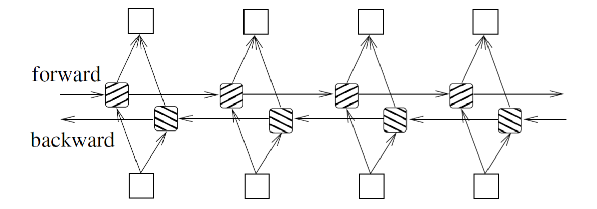
Bidirectional LSTMs

A Recurrent Neural Network (RNN) is a feedforward neural network with internal memory. As it performs the same function for every input of data, an RNN is recurrent in nature while the output of the current input depends on the past one.

Bidirectional LSTM is a type of RNN with better results for long sequences and better memory, preserving the context along with the time series. Bidirectional LSTMs train two, instead of one, LSTMs on the input sequence in problems where all timesteps of the input sequence are available by traversing from both directions as illustrated below.

Here is our Model architecture for the problem.

from keras.layers import Dense, Embedding, LSTM, Bidirectional, Input
from keras.models import Model

def make_model(max_length,embedding_matrix):

    # Defining the embedding layer
    embedding_dim = 64 
    input1=Input(shape=(max_length,))
    
    embedding_layer = Embedding(len(word_index) + 1,
                                100,
                                weights=[embedding_matrix],
                                input_length=max_length,
                                trainable=False)(input1)
                                
    # Building LSTM for text features                          
    bi_lstm_1 = Bidirectional(LSTM(embedding_dim,return_sequences=True))(embedding_layer)
    
    bi_lstm_2 = Bidirectional(LSTM(embedding_dim))(bi_lstm_1)   
    lstm_output =  Model(inputs = input1,outputs = bi_lstm_2)
    
    #Inputting Number features
    input2=Input(shape=(9,))  
    
    # Merging inputs
    merge = concatenate([lstm_output.output,input2])
    
    # Building dense layers for regression with number features
    reg_dense1 = Dense(64, activation='relu')(merge)
    reg_dense2 = Dense(16, activation='relu')(reg_dense1) 
    output1 = Dense(1, activation='sigmoid')(reg_dense2)
    
    # Building dense layers for classification with number features
    clf_dense1 = Dense(64, activation='relu')(merge)
    clf_dense2 = Dense(16, activation='relu')(clf_dense1)
    
    # 5 Categories in classification
    output2 = Dense(5, activation='softmax')(clf_dense2)
 
    model = Model(inputs=[lstm_output.input,input2], outputs=[output1,output2])
 
    return model

Model Summary

Layer (type)                    Output Shape         Param #  
   Connected to
==============================================================================
input_1 (InputLayer)            [(None, 2150)]       0        

______________________________________________________________________________
embedding (Embedding)           (None, 2150, 100)    1368500  
   input_1[0][0]
______________________________________________________________________________
bidirectional (Bidirectional)   (None, 2150, 128)    84480    
   embedding[0][0]
______________________________________________________________________________
bidirectional_1 (Bidirectional) (None, 128)          98816    
   bidirectional[0][0]
______________________________________________________________________________
input_2 (InputLayer)            [(None, 9)]          0        

______________________________________________________________________________
concatenate (Concatenate)       (None, 137)          0        
   bidirectional_1[0][0]

   input_2[0][0]
______________________________________________________________________________
dense (Dense)                   (None, 64)           8832     
   concatenate[0][0]
______________________________________________________________________________
dense_3 (Dense)                 (None, 64)           8832     
   concatenate[0][0]
______________________________________________________________________________
dense_1 (Dense)                 (None, 16)           1040     
   dense[0][0]
______________________________________________________________________________
dense_4 (Dense)                 (None, 16)           1040     
   dense_3[0][0]
______________________________________________________________________________
dense_2 (Dense)                 (None, 1)            17       
   dense_1[0][0]
______________________________________________________________________________
dense_5 (Dense)                 (None, 5)            85          dense_4[0][0]
==============================================================================
Total params: 1,571,642
Trainable params: 203,142
Non-trainable params: 1,368,500

The model summary might look intimidating given that we have multiple inputs and outputs. Let’s visualize the model to get a big picture.

Model Visualization

Now, all that we have left to do is to compile and fit the model. Let’s see how different it is from a normal case. We can input arrays for our model's input and output values.

import keras
from keras.optimizers import Adam

model = make_model(max_length,embedding_matrix)
    
# Defining losses for each output
losses ={ 'dense_2':keras.losses.MeanSquaredError(),
    'dense_5':keras.losses.CategoricalCrossentropy()}
 
opt = Adam(lr=0.01)

# Model Compiling
model.compile(optimizer=opt, loss=losses,metrics="accuracy")

# Model Fitting
H = model.fit(x=[X_text_train_padded, X_num_train],
y={'dense_2': y_reg_train, 'dense_5': y_clf_train},
	validation_data=([X_text_val_padded, X_num_val],
    	{'dense_2': y_reg_val, 'dense_5': y_clf_val}), epochs=10,verbose=1)

That's all there is to it!

Conclusion

Keras Functional API helps us in building such robust and powerful models, so the possibilities are truly vast and exciting. Getting better control over inputs, outputs, layers and the flow helps one to engineer models with high levels of precision and flexibility. I encourage you all to try out varying layers, parameters, and everything possible to get the best out of these features using Hypertuning.

Good luck with your own experiments and thanks for reading!