Hello again in the series of tutorials for implementing a generic gradient descent (GD) algorithm in Python for optimizing parameters of artificial neural network (ANN) in the backpropagation phase. The GD implementation will be generic and can work with any ANN architecture. This is the second tutorial in the series which discusses extending the implementation of Part 1 for allowing the GD algorithm to work with any number of inputs in the input layer.

This tutorial, which is Part 2 of the series, has 2 sections. Each section discusses building the GD algorithm for architecture with a different number of inputs. The first architecture, the number of input neurons is 2. The second one will include 10 neurons. Through these examples, we can deduce some generic rules for implementing the GD algorithm that can work with any number of inputs.

2 Inputs – 1 Output

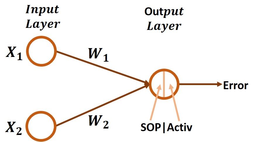
This section extends the implementation of the GD algorithm in Part 1 to allow it to work with an input layer with 2 inputs rather than just 1 input. The diagram of the ANN with 2 inputs and 1 output is given in the next figure. Now, each input will have a different weight. For the first input X1, there is a weight W1. For the second input X2, its weight is W2. How to allow the GD algorithm to work with these 2 parameters? The answer will be much simpler after writing the chain of the error to W1 and W2 derivatives.

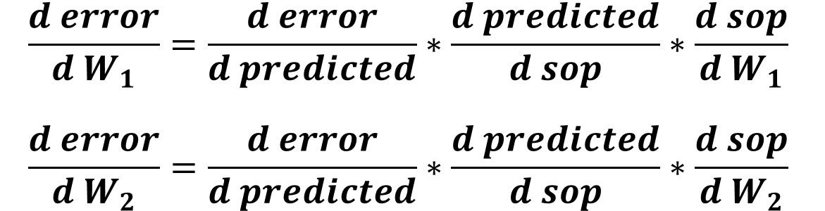
The derivative chain for the error to W1 and W2 are given in the next figure. What is the difference? The difference is how to calculate the last derivative between the SOP and the weight. The first 2 derivatives are identical for both W1 and W2.

The code listed below gives the implementation for calculating the above derivatives. There are 3 major differences compared to Part 1 implementation.

The first one is that there are 2 lines of code for initializing the 2 weights using numpy.random.rand().

The second change is that the SOP is calculated as the sum of products between each input and its associated weight (X1*W1+X2*W2).

The third change is calculating the derivative of the SOP to each of the 2 weights. In Part 1, there was just a single weight and thus a single derivative was calculated. In this example, you can think of it as just doubling the lines of code. The variable g3w1 calculates the derivative for W1 and the variable g3w2 calculates the derivative for W2. Finally, the gradient by which each weight is updated is calculated in the 2 variables gradw1 and gradw2. Finally, 2 calls to the update_w() function for updating each weight.

import numpy

def sigmoid(sop):
    return 1.0/(1+numpy.exp(-1*sop))

def error(predicted, target):
    return numpy.power(predicted-target, 2)

def error_predicted_deriv(predicted, target):
    return 2*(predicted-target)

def activation_sop_deriv(sop):
    return sigmoid(sop)*(1.0-sigmoid(sop))

def sop_w_deriv(x):
    return x

def update_w(w, grad, learning_rate):
    return w - learning_rate*grad

x1=0.1
x2=0.4
target = 0.3
learning_rate = 0.1
w1=numpy.random.rand()
w2=numpy.random.rand()
print("Initial W : ", w1, w2)

# Forward Pass
y = w1*x1 + w2*x2
predicted = sigmoid(y)
err = error(predicted, target)
    
# Backward Pass
g1 = error_predicted_deriv(predicted, target)

g2 = activation_sop_deriv(predicted)
    
g3w1 = sop_w_deriv(x1)
g3w2 = sop_w_deriv(x2)
    
gradw1 = g3w1*g2*g1
gradw2 = g3w2*g2*g1
    
w1 = update_w(w1, gradw1, learning_rate)
w2 = update_w(w2, gradw2, learning_rate)

print(predicted)

The previous code just works for 1 iteration. We can use a loop to go through a number of iterations in which the weighs can be updated to a better value. Here is the new code.

import numpy

def sigmoid(sop):
    return 1.0/(1+numpy.exp(-1*sop))

def error(predicted, target):
    return numpy.power(predicted-target, 2)

def error_predicted_deriv(predicted, target):
    return 2*(predicted-target)

def activation_sop_deriv(sop):
    return sigmoid(sop)*(1.0-sigmoid(sop))

def sop_w_deriv(x):
    return x

def update_w(w, grad, learning_rate):
    return w - learning_rate*grad

x1=0.1
x2=0.4
target = 0.3
learning_rate = 0.1
w1=numpy.random.rand()
w2=numpy.random.rand()
print("Initial W : ", w1, w2)

for k in range(80000):
    # Forward Pass
    y = w1*x1 + w2*x2
    predicted = sigmoid(y)
    err = error(predicted, target)
    
    # Backward Pass
    g1 = error_predicted_deriv(predicted, target)

    g2 = activation_sop_deriv(predicted)
    
    g3w1 = sop_w_deriv(x1)
    g3w2 = sop_w_deriv(x2)
    
    gradw1 = g3w1*g2*g1
    gradw2 = g3w2*g2*g1
    
    w1 = update_w(w1, gradw1, learning_rate)
    w2 = update_w(w2, gradw2, learning_rate)

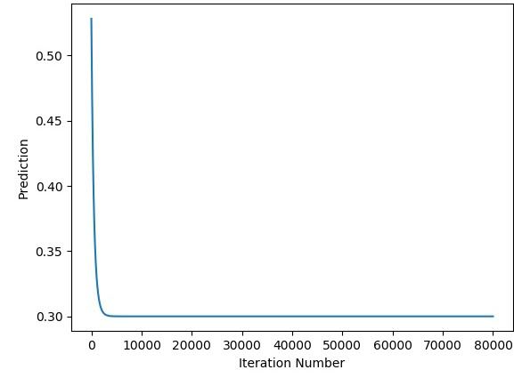
    print(predicted)

The figure below shows how the prediction of the ANN changes until reaching the desired output which is 0.3. After around 5,000 iterations, the network is able to do the correct prediction.

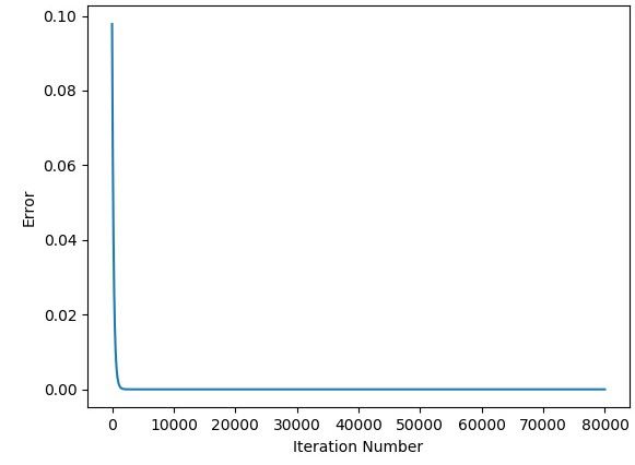
The next figure shows how the error changes by the iteration number. The error is 0.0 after 5,000 iterations.

Up to this point, we successfully implemented the GD algorithm for working with either 1 input or 2 inputs. In the next section, the previous implementation will be extended to allow the algorithm to work with 10 inputs.

10 Inputs – 1 Output

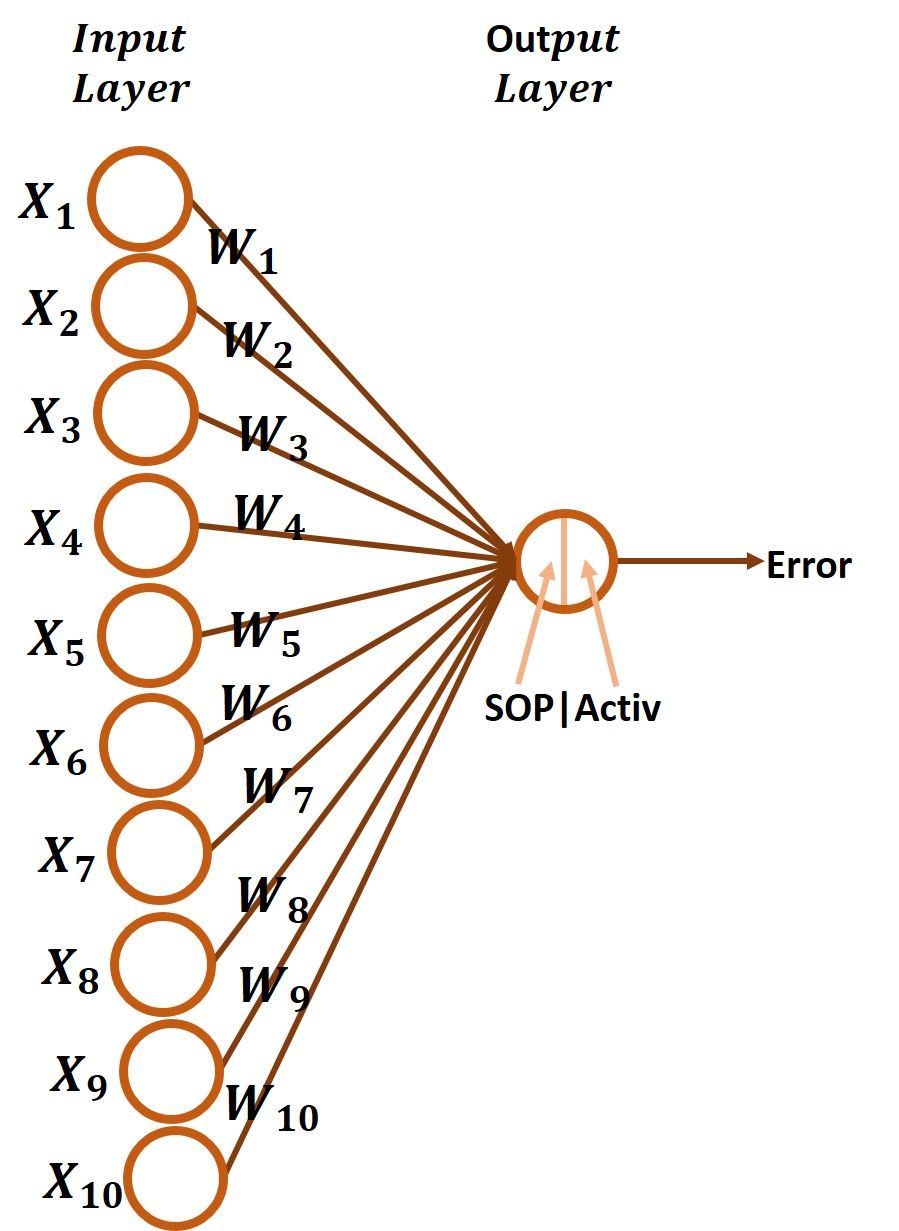
The network architecture with 10 inputs and 1 output is given below. There are 10 inputs X1 to X10 and 10 weights W1 to W10 and each input has its weight. Building the GD algorithm for training such a network is similar to the previous example but just using 10 inputs rather than 2. It is just a matter of repeating the lines of code that calculate the derivative between the SOP and each weight.

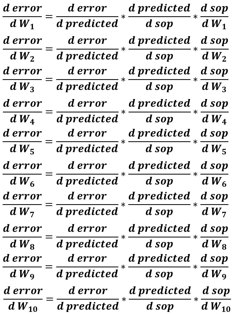
Before writing the code for calculating the derivatives, it is better to list the necessary derivatives to be calculated which are summarized in the next figure. It is clear that the first 2 derivatives are fixed across all weights but the last derivative (SOP to weight derivative) is what changes for each weight.

In the previous example, there were just 2 weights and thus there were the following:

1. 2 lines of code for specifying the value of each of the 2 inputs.
2. 2 lines of code for initializing the 2 weights.
3. Calculating the SOP by summing the product between the 2 inputs and the 2 weights.
4. 2 lines of code for calculating the SOP and to the 2 weights derivatives.
5. 2 lines for calculating the gradient for the 2 weights.
6. 2 lines for updating the 2 weights.

In this example, 10 lines will replace the 2 lines and thus the following will be existing:

1. 10 lines of code for specifying the value of each of the 10 inputs.
2. 10 lines of code for initializing the 10 weights.
3. Calculating the SOP by summing the product between the 10 inputs and the 10 weights.
4. 10 lines of code for calculating the SOP to the 10 weights derivatives.
5. 10 lines for calculating the gradient for the 10 weights.
6. 10 lines for updating the 10 weights.

The code for implementing the GD algorithm for a network with 10 inputs is given below.

import numpy

def sigmoid(sop):
    return 1.0/(1+numpy.exp(-1*sop))

def error(predicted, target):
    return numpy.power(predicted-target, 2)

def error_predicted_deriv(predicted, target):
    return 2*(predicted-target)

def sigmoid_sop_deriv(sop):
    return sigmoid(sop)*(1.0-sigmoid(sop))

def sop_w_deriv(x):
    return x

def update_w(w, grad, learning_rate):
    return w - learning_rate*grad

x1=0.1
x2=0.4
x3=4.1
x4=4.3
x5=1.8
x6=2.0
x7=0.01
x8=0.9
x9=3.8
x10=1.6

target = 0.3
learning_rate = 0.01

w1=numpy.random.rand()
w2=numpy.random.rand()
w3=numpy.random.rand()
w4=numpy.random.rand()
w5=numpy.random.rand()
w6=numpy.random.rand()
w7=numpy.random.rand()
w8=numpy.random.rand()
w9=numpy.random.rand()
w10=numpy.random.rand()

print("Initial W : ", w1, w2, w3, w4, w5, w6, w7, w8, w9, w10)

# Forward Pass
y = w1*x1 + w2*x2 + w3*x3 + w4*x4 + w5*x5 + w6*x6 + w7*x7 + w8*x8 + w9*x9 + w10*x10
predicted = sigmoid(y)
err = error(predicted, target)
    
# Backward Pass
g1 = error_predicted_deriv(predicted, target)

g2 = sigmoid_sop_deriv(y)
    
g3w1 = sop_w_deriv(x1)
g3w2 = sop_w_deriv(x2)
g3w3 = sop_w_deriv(x3)
g3w4 = sop_w_deriv(x4)
g3w5 = sop_w_deriv(x5)
g3w6 = sop_w_deriv(x6)
g3w7 = sop_w_deriv(x7)
g3w8 = sop_w_deriv(x8)
g3w9 = sop_w_deriv(x9)
g3w10 = sop_w_deriv(x10)
    
gradw1 = g3w1*g2*g1
gradw2 = g3w2*g2*g1
gradw3 = g3w3*g2*g1
gradw4 = g3w4*g2*g1
gradw5 = g3w5*g2*g1
gradw6 = g3w6*g2*g1
gradw7 = g3w7*g2*g1
gradw8 = g3w8*g2*g1
gradw9 = g3w9*g2*g1
gradw10 = g3w10*g2*g1
    
w1 = update_w(w1, gradw1, learning_rate)
w2 = update_w(w2, gradw2, learning_rate)
w3 = update_w(w3, gradw3, learning_rate)
w4 = update_w(w4, gradw4, learning_rate)
w5 = update_w(w5, gradw5, learning_rate)
w6 = update_w(w6, gradw6, learning_rate)
w7 = update_w(w7, gradw7, learning_rate)
w8 = update_w(w8, gradw8, learning_rate)
w9 = update_w(w9, gradw9, learning_rate)
w10 = update_w(w10, gradw10, learning_rate)

print(predicted)

As regular, the previous code just goes through a single iteration. We can use a loop to train the network in a number of iterations.

import numpy

def sigmoid(sop):
    return 1.0/(1+numpy.exp(-1*sop))

def error(predicted, target):
    return numpy.power(predicted-target, 2)

def error_predicted_deriv(predicted, target):
    return 2*(predicted-target)

def sigmoid_sop_deriv(sop):
    return sigmoid(sop)*(1.0-sigmoid(sop))

def sop_w_deriv(x):
    return x

def update_w(w, grad, learning_rate):
    return w - learning_rate*grad

x1=0.1
x2=0.4
x3=4.1
x4=4.3
x5=1.8
x6=2.0
x7=0.01
x8=0.9
x9=3.8
x10=1.6

target = 0.3
learning_rate = 0.01

w1=numpy.random.rand()
w2=numpy.random.rand()
w3=numpy.random.rand()
w4=numpy.random.rand()
w5=numpy.random.rand()
w6=numpy.random.rand()
w7=numpy.random.rand()
w8=numpy.random.rand()
w9=numpy.random.rand()
w10=numpy.random.rand()

print("Initial W : ", w1, w2, w3, w4, w5, w6, w7, w8, w9, w10)

for k in range(1000000000):
    # Forward Pass
    y = w1*x1 + w2*x2 + w3*x3 + w4*x4 + w5*x5 + w6*x6 + w7*x7 + w8*x8 + w9*x9 + w10*x10
    predicted = sigmoid(y)
    err = error(predicted, target)
    
    # Backward Pass
    g1 = error_predicted_deriv(predicted, target)

    g2 = sigmoid_sop_deriv(y)
    
    g3w1 = sop_w_deriv(x1)
    g3w2 = sop_w_deriv(x2)
    g3w3 = sop_w_deriv(x3)
    g3w4 = sop_w_deriv(x4)
    g3w5 = sop_w_deriv(x5)
    g3w6 = sop_w_deriv(x6)
    g3w7 = sop_w_deriv(x7)
    g3w8 = sop_w_deriv(x8)
    g3w9 = sop_w_deriv(x9)
    g3w10 = sop_w_deriv(x10)
    
    gradw1 = g3w1*g2*g1
    gradw2 = g3w2*g2*g1
    gradw3 = g3w3*g2*g1
    gradw4 = g3w4*g2*g1
    gradw5 = g3w5*g2*g1
    gradw6 = g3w6*g2*g1
    gradw7 = g3w7*g2*g1
    gradw8 = g3w8*g2*g1
    gradw9 = g3w9*g2*g1
    gradw10 = g3w10*g2*g1
    
    w1 = update_w(w1, gradw1, learning_rate)
    w2 = update_w(w2, gradw2, learning_rate)
    w3 = update_w(w3, gradw3, learning_rate)
    w4 = update_w(w4, gradw4, learning_rate)
    w5 = update_w(w5, gradw5, learning_rate)
    w6 = update_w(w6, gradw6, learning_rate)
    w7 = update_w(w7, gradw7, learning_rate)
    w8 = update_w(w8, gradw8, learning_rate)
    w9 = update_w(w9, gradw9, learning_rate)
    w10 = update_w(w10, gradw10, learning_rate)

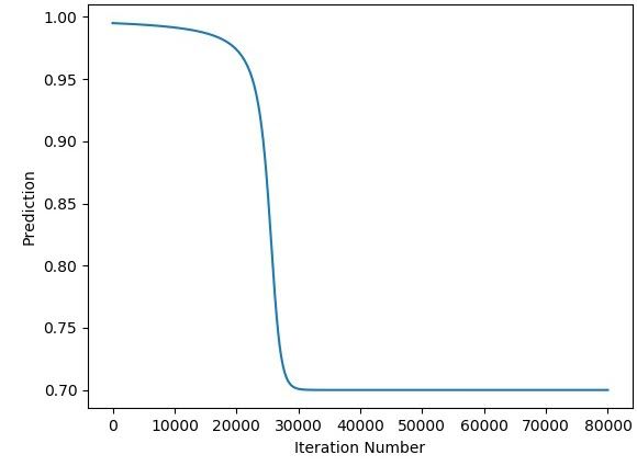
    print(predicted)

The next figure shows how the predicted output changes by the iteration number.

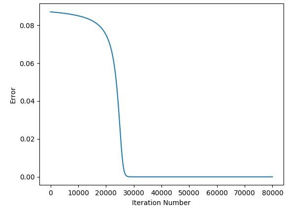
The next figure shows the relationship between the error and the iteration number. The error is 0.0 after around 26,000 iterations.

Up to this point, the implementation of the GD algorithm for optimizing a network with 10 inputs is complete. You might wonder what if there are more than 10 inputs. Do we have to add more lines for each input neuron? Using the current implementation, we have to duplicate the lines but it is not the only way to do. We can refine the previous code so that there is no need to modify the code at all for working with any number of inputs.

Working with any Number of Inputs

The strategy followed at the current time for implementing the GD algorithm is to duplicate some lines code for each new input. Despite being a legacy way to do, but it is helpful to understand how each little step works. In this section, the previous implementation will be refined so that we do not have to edit the code when the number of inputs increases or decreases. What we are going to do is to inspect the previous implementation for the lines that repeat for each input neuron. After that, these lines will be replaced by just a single line that works for all inputs. In the previous code, there are 6 parts to be refined:

1. Specifying inputs values.
2. Weights initialization.
3. Calculating the SOP.
4. Calculating the SOP to Weights Derivatives.
5. Calculating the gradients of the weights.
6. Updating the weights.

Let's work with each part and see what we can do.

Specifying Inputs Values

The part of the previous code used for specifying the values of all inputs is as given below. If more inputs are to be added, more lines will be written.

x1=0.1
x2=0.4
x3=1.1
x4=1.3
x5=1.8
x6=2.0
x7=0.01
x8=0.9
x9=0.8
x10=1.6

We can use a better approach by replacing all of these lines by just the single line given below. A NumPy array holds all of these inputs. Using indexing, we can return all individual inputs. For example, if the first input is to be retrieved, then index 0 is used for indexing the array x.

x = numpy.array([0.1, 0.4, 1.1, 1.3, 1.8, 2.0, 0.01, 0.9, 0.8, 1.6])

Weights Initialization

The part of the previous code used for initializing the weights is given below. If more weights are to be initialized, more lines will be written.

w1=numpy.random.rand()
w2=numpy.random.rand()
w3=numpy.random.rand()
w4=numpy.random.rand()
w5=numpy.random.rand()
w6=numpy.random.rand()
w7=numpy.random.rand()
w8=numpy.random.rand()
w9=numpy.random.rand()
w10=numpy.random.rand()

Rather than adding a separate line for initializing each weight, we can replace all of these lines by the line below. This returns a NumPy array with 10 values, one for each weight. Again, using indexing we can retrieve the individual weights.

w = numpy.random.rand(10)

Calculating the SOP

The SOP in the previous code was calculated as given below. For each input, we have to add a new term to the equation below for multiplying it by its weight.

y = w1*x1 + w2*x2 + w3*x3 + w4*x4 + w5*x5 + w6*x6 + w7*x7 + w8*x8 + w9*x9 + w10*x10

Rather than multiplying each input by its weight this way, we can use a better approach. Remember that the SOP is calculated by multiplying each input by its weight. Also, remember that both x and ware now NumPy arrays and each has 10 values where the weight at index iin array w corresponds to the input at index i at array x. What we need is multiplying each input by its weight and return the sum of these multiplications. The good news is that NumPy supports multiplying arrays value by value. Thus, writing w*x will return a new array with 10values representing the product of each input by its weight. We can sum all of these products and return the SOP using the line given below.

y = numpy.sum(w*x)

Calculating the SOP to Weights Derivatives

The next part of the code that needs to be edited is the part responsible for calculating the SOP to weights derivatives. It is given below.

g3w1 = sop_w_deriv(x1)
g3w2 = sop_w_deriv(x2)
g3w3 = sop_w_deriv(x3)
g3w4 = sop_w_deriv(x4)
g3w5 = sop_w_deriv(x5)
g3w6 = sop_w_deriv(x6)
g3w7 = sop_w_deriv(x7)
g3w8 = sop_w_deriv(x8)
g3w9 = sop_w_deriv(x9)
g3w10 = sop_w_deriv(x10)

Rather than calling the sop_w_deriv() function for calculating the derivative for each weight, we can simply pass the array x to this function as given below. When this function receives a NumPy array, it processes each value in that array independently and returns a new NumPy array with the result.

g3 = sop_w_deriv(x)

Calculating the Gradients of the Weights

The code part responsible for calculating the gradients of the weights is given below.

gradw1 = g3w1*g2*g1
gradw2 = g3w2*g2*g1
gradw3 = g3w3*g2*g1
gradw4 = g3w4*g2*g1
gradw5 = g3w5*g2*g1
gradw6 = g3w6*g2*g1
gradw7 = g3w7*g2*g1
gradw8 = g3w8*g2*g1
gradw9 = g3w9*g2*g1
gradw10 = g3w10*g2*g1

Rather than adding a new line for multiplying all derivatives in the chain for each weight, we can simply use the line below. Remember that both g1 and g2 are arrays holding a single value but g3 is a Numpy array holding 10 values. This can be regarded as multiplying an array with a scalar value.

grad = g3*g2*g1

Updating the Weights

The final code part to be edited is listed below which is responsible for updating the weights.

w1 = update_w(w1, gradw1, learning_rate)
w2 = update_w(w2, gradw2, learning_rate)
w3 = update_w(w3, gradw3, learning_rate)
w4 = update_w(w4, gradw4, learning_rate)
w5 = update_w(w5, gradw5, learning_rate)
w6 = update_w(w6, gradw6, learning_rate)
w7 = update_w(w7, gradw7, learning_rate)
w8 = update_w(w8, gradw8, learning_rate)
w9 = update_w(w9, gradw9, learning_rate)
w10 = update_w(w10, gradw10, learning_rate)

Rather than calling the update_w() function for each weight, we can simply pass the grad array calculated in the previous step alongside with the weights array w to this function as given below. Inside the function, the weights update equation will be called for each weight and its gradient. It will return a new array of 10 values representing the new weights that can be used in the next iteration.

w = update_w(w, grad, learning_rate)

After making all edits, the final optimized code is given below. It shows the previous code but commented as a way of mapping each part with its edit.

import numpy

def sigmoid(sop):
    return 1.0/(1+numpy.exp(-1*sop))

def error(predicted, target):
    return numpy.power(predicted-target, 2)

def error_predicted_deriv(predicted, target):
    return 2*(predicted-target)

def sigmoid_sop_deriv(sop):
    return sigmoid(sop)*(1.0-sigmoid(sop))

def sop_w_deriv(x):
    return x

def update_w(w, grad, learning_rate):
    return w - learning_rate*grad

#x1=0.1
#x2=0.4
#x3=4.1
#x4=4.3
#x5=1.8
#x6=2.0
#x7=0.01
#x8=0.9
#x9=3.8
#x10=1.6
x = numpy.array([0.1, 0.4, 1.1, 1.3, 1.8, 2.0, 0.01, 0.9, 0.8, 1.6])
target = numpy.array([0.2])

learning_rate = 0.1

#w1=numpy.random.rand()
#w2=numpy.random.rand()
#w3=numpy.random.rand()
#w4=numpy.random.rand()
#w5=numpy.random.rand()
#w6=numpy.random.rand()
#w7=numpy.random.rand()
#w8=numpy.random.rand()
#w9=numpy.random.rand()
#w10=numpy.random.rand()
w = numpy.random.rand(10)

#print("Initial W : ", w1, w2, w3, w4, w5, w6, w7, w8, w9, w10)
print("Initial W : ", w)

for k in range(1000000000):
    # Forward Pass
#    y = w1*x1 + w2*x2 + w3*x3 + w4*x4 + w5*x5 + w6*x6 + w7*x7 + w8*x8 + w9*x9 + w10*x10
    y = numpy.sum(w*x)
    predicted = sigmoid(y)
    err = error(predicted, target)
    
    # Backward Pass
    g1 = error_predicted_deriv(predicted, target)

    g2 = sigmoid_sop_deriv(y)
    
#    g3w1 = sop_w_deriv(x1)
#    g3w2 = sop_w_deriv(x2)
#    g3w3 = sop_w_deriv(x3)
#    g3w4 = sop_w_deriv(x4)
#    g3w5 = sop_w_deriv(x5)
#    g3w6 = sop_w_deriv(x6)
#    g3w7 = sop_w_deriv(x7)
#    g3w8 = sop_w_deriv(x8)
#    g3w9 = sop_w_deriv(x9)
#    g3w10 = sop_w_deriv(x10)
    g3 = sop_w_deriv(x)
#    g3 = numpy.array([sop_w_deriv(x_) for x_ in x])
    
#    gradw1 = g3w1*g2*g1
#    gradw2 = g3w2*g2*g1
#    gradw3 = g3w3*g2*g1
#    gradw4 = g3w4*g2*g1
#    gradw5 = g3w5*g2*g1
#    gradw6 = g3w6*g2*g1
#    gradw7 = g3w7*g2*g1
#    gradw8 = g3w8*g2*g1
#    gradw9 = g3w9*g2*g1
#    gradw10 = g3w10*g2*g1
    grad = g3*g2*g1
    
#    w1 = update_w(w1, gradw1, learning_rate)
#    w2 = update_w(w2, gradw2, learning_rate)
#    w3 = update_w(w3, gradw3, learning_rate)
#    w4 = update_w(w4, gradw4, learning_rate)
#    w5 = update_w(w5, gradw5, learning_rate)
#    w6 = update_w(w6, gradw6, learning_rate)
#    w7 = update_w(w7, gradw7, learning_rate)
#    w8 = update_w(w8, gradw8, learning_rate)
#    w9 = update_w(w9, gradw9, learning_rate)
#    w10 = update_w(w10, gradw10, learning_rate)
    w = update_w(w, grad, learning_rate)
#    w = numpy.array([update_w(w_, grad_, learning_rate) for (w_, grad_) in [(w[i], grad[i]) for i in range(10)]])

    print(predicted)

After removing the comments, the code is given below. The code is now very clear.

import numpy

def sigmoid(sop):
    return 1.0/(1+numpy.exp(-1*sop))

def error(predicted, target):
    return numpy.power(predicted-target, 2)

def error_predicted_deriv(predicted, target):
    return 2*(predicted-target)

def sigmoid_sop_deriv(sop):
    return sigmoid(sop)*(1.0-sigmoid(sop))

def sop_w_deriv(x):
    return x

def update_w(w, grad, learning_rate):
    return w - learning_rate*grad

x = numpy.array([0.1, 0.4, 1.1, 1.3, 1.8, 2.0, 0.01, 0.9, 0.8, 1.6])
target = numpy.array([0.2])

learning_rate = 0.1

w = numpy.random.rand(10)

print("Initial W : ", w)

for k in range(1000000000):
    # Forward Pass
    y = numpy.sum(w*x)
    predicted = sigmoid(y)
    err = error(predicted, target)
    
    # Backward Pass
    g1 = error_predicted_deriv(predicted, target)

    g2 = sigmoid_sop_deriv(y)
    
    g3 = sop_w_deriv(x)

    grad = g3*g2*g1
    
    w = update_w(w, grad, learning_rate)

    print(predicted)

Suppose that we are looking to create a network with 5 inputs, we can simply make 2 changes:

1. Preparing the input array xto just have 5 values.
2. Replacing 10 by 5 inside numpy.random.rand().

The code that works for 5 inputs is given below.

import numpy

def sigmoid(sop):
    return 1.0/(1+numpy.exp(-1*sop))

def error(predicted, target):
    return numpy.power(predicted-target, 2)

def error_predicted_deriv(predicted, target):
    return 2*(predicted-target)

def sigmoid_sop_deriv(sop):
    return sigmoid(sop)*(1.0-sigmoid(sop))

def sop_w_deriv(x):
    return x

def update_w(w, grad, learning_rate):
    return w - learning_rate*grad

x = numpy.array([0.1, 0.4, 1.1, 1.3, 1.8])
target = numpy.array([0.2])

learning_rate = 0.1

w = numpy.random.rand(5)

print("Initial W : ", w)

for k in range(1000000000):
    # Forward Pass
    y = numpy.sum(w*x)
    predicted = sigmoid(y)
    err = error(predicted, target)
    
    # Backward Pass
    g1 = error_predicted_deriv(predicted, target)

    g2 = sigmoid_sop_deriv(y)
    
    g3 = sop_w_deriv(x)

    grad = g3*g2*g1
    
    w = update_w(w, grad, learning_rate)

    print(predicted)

Conclusion

At this point, we successfully implemented the GD algorithm for working with an ANN with an input layer and an output layer where the input layer can include any number of inputs. In the next tutorial, this implementation will be extended to add a single hidden layer to the ANN and be optimized using the GD algorithm.