Hello again in the series of tutorials for implementing a generic gradient descent (GD) algorithm in Python for optimizing parameters of artificial neural network (ANN) in the backpropagation phase. The GD implementation will be generic and can work with any ANN architecture.

In Part 2, the GD algorithm is implemented so that it can work with any number of input neurons. In Part 3, which is the third tutorial in the series, the implementation of Part 2 will be extended for allowing the GD algorithm to work with a single hidden layer with 2 neurons. This tutorial has 2 sections. In the first section, the ANN will have 3 inputs, 1 hidden layer with 3 neurons, and an output layer with one neuron. In the second section, the number of inputs will be increased from 3 to 10.

1 Hidden Layer with 2 Neurons

This section extends the implementation of the GD algorithm in Part 2 to allow it to work with a hidden layer with 2 neurons. Part 2 was using 10 inputs but for simplicity, just 3 inputs will be used in this section. The diagram of the ANN with 3 inputs, 1 hidden layer with 2 neurons, and 1 output neuron is given in the next figure.

Now, each input of the 3 inputs is connected to the 2 hidden neurons. For each connection, there is a different weight. The weights between the input and hidden layer are labeled as Wzy where z refers to the input layer neuron index and y refers to the index of the hidden neuron.

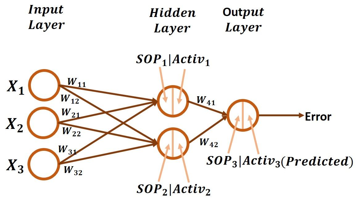
The weight for the connection between the first input X1and the first hidden neuron is W11. Also, weight W12 is for the connection between X1 and the second hidden neuron. Regarding X2, the weights W21 and W22 are for the connections to the first and second hidden neuron, respectively. Similarly, X3 has 2 weights W31and W32.

In addition to the weights between the input and hidden layers, there are 2 weights connecting the 2 hidden neurons to the output neuron which are W41 and W42.

How to allow the GD algorithm to work with all of these parameters? The answer will be much simpler after writing the chain of derivatives starting from the error until reaching each individual weight. As regular, before thinking of the backward pass in which the GD algorithm updates the weights, we have to start by the forward pass.

Forward Pass

In the forward pass, the neurons in the hidden layer accept the inputs from the input layer in addition to their weights. Then, the sum of products (SOP) between the inputs and their weights is calculated. Regarding the first hidden neuron, it accepts the 3 inputs X1, X2, and X3 in addition to their weights W11, W21, and W31, respectively. The SOP for this neuron is calculated by summing the products between each input and its weight and thus the result is:

SOP1=X1*W11+X2*W21+X3*W31

The SOP for the first hidden neuron is labeled SOP1 in the figure for reference. For the second hidden neuron, its SOP, which is labeled SOP2, is as follows:

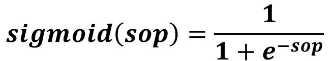
SOP2=X1*W12+X2*W22+X3*W32

After calculating the SOP for all hidden neurons, next is to feed such SOP to the activation function. The function used in this series is the sigmoid function which is calculated as given in the equation in the next figure.

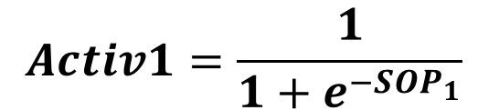
By feeding SOP1 to the sigmoid function, the result is Activ1 as calculated by the next equation:

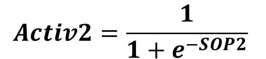
It is Activ2 for the SOP2 as calculated by the next equation:

Remember that in the forward pass the outputs of a layer are regarded as the inputs to the next layer. Such the outputs of the hidden layer which are Activ1 and Activ2 are regarded as the inputs to the output layer. The process repeats for calculating the SOP in the output layer neuron. Each input to the output neuron has a weight. For the first input Activ1, its weight is W41. The weight for the second input Activ2 is W42. The SOP for the output neuron is labeled SOP3 and calculated as follows:

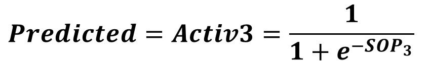
SOP3=Activ1*W41+Activ2*W42

SOP3 is fed to the sigmoid function to return Activ3as given in the next equation:

In this tutorial, the output of the activation function is regarded as the predicted output of the network. After the network makes a prediction, next is to calculate the error using the squared error function given below.

At this point, the forward pass is complete and we are ready to go through the backward pass.

Backward Pass

In the backward pass, the goal is to calculate the gradient that updates each weight in the network. Because we start from where we ended in the forward pass, the gradient for the last layer is calculated at first then move until reaching the input layer. Let's start calculating the gradients of weights between the hidden layer and the output layer.

Because there is no explicit equation that includes both the error and the weights (W41 and W42), then it is preferred to use the chain rule. What is the chain of derivatives that are necessary to calculate the gradients for such weights?

Starting by the first weight, we need to find the derivative of the error to W41. The error equation has 2 terms as follows:

1. Predicted
2. Target

Of these 2 terms, which one links the error to the weight W41? Sure it is Predicted because it is calculated using the sigmoid function which accepts SOP3 which includes W41. Thus, the first derivative to calculate is the error to predicted output derivative which is calculated as given in the next equation.

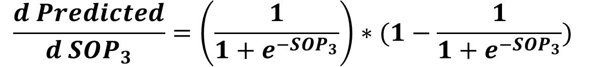
After that, next is to calculate the Predicted to SOP3derivative by substituting in the derivative of the sigmoid function by SOP3as given in the next equation.

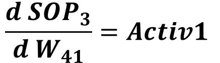
Next is to calculate the SOP3 to W41 derivative. Remember the equation that includes both SOP3 and W41. It is repeated below.

SOP3 = Activ1*W41 + Activ2*W42

The derivative of SOP3 to W41 is given in the next equation.

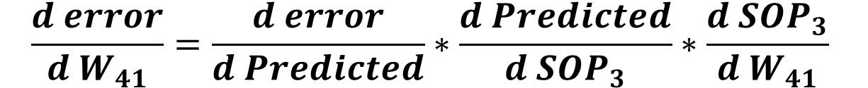
By calculating all derivatives in the chain from the error to W41, we can calculate the error to W41 derivative by multiplying all of these derivatives as given in the next equation.

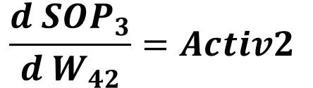
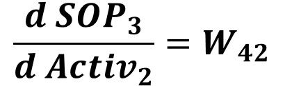
Similar to calculating the error to W41derivative, we can easily calculate the error to W42 derivative. The only term that will change from the previous equation is the last one. Rather than calculating the SOP3 to W41 derivative, now we calculate the SOP3 to W42 derivative which is given in the next equation.

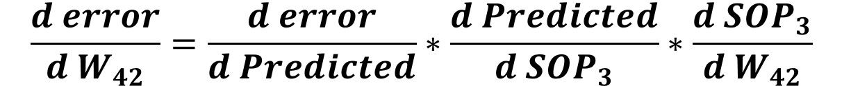
Finally, the error to W42 derivative is calculated according to the next equation.

At this point, we successfully calculated the gradients for all weights between the hidden layer and the output layer. Next is to calculate the gradients for the weights between the input layer and the hidden layer. What is the derivative chain between the error and the weights between such 2 layers? For sure, the first 2 derivatives are the first 2 ones used in the previous chain which are as follows:

1. Error to the Predicted derivative.
2. Predicted to SOP3 derivative.

Rather than calculating the SOP3 to W41 and W4s derivatives, we need to calculate the SOP3 to Activ1 and Activ2 derivatives. SOP3 to Activ1 derivative helps to calculate the gradients of the weights connected to the first hidden neuron which are W11, W21, and W31. SOP3 to Activ2 derivative helps to calculate the gradients of the weights connected to the second hidden neuron which are W12, W22, and W32.

Starting by Activ1, the equation relating SOP3 to Activ1 is repeated below:

SOP3=Activ1*W41+Activ2*W42

The SOP3 to Activ1 derivative is calculated as given in the next equation:

Similarly, the SOP3 to Activ2 derivative is calculated as given in the next equation:

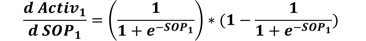
After that, we can calculate the next derivative in the chain which is Activ1 to SOP1 derivative which is calculated by substituting by SOP1 in the derivative equation of the sigmoid function as follows. This will be used for updating the weights W11, W21, and W31.

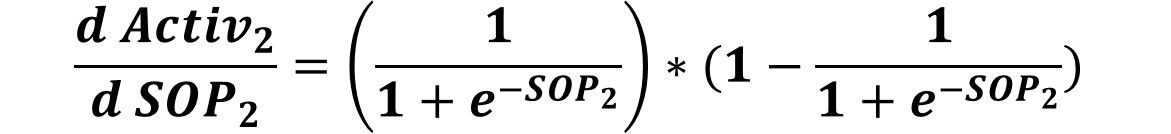
Similarly, the Activ2 to SOP2 derivative is calculated as follows. This will be used for updating the weights W12, W22, and W32.

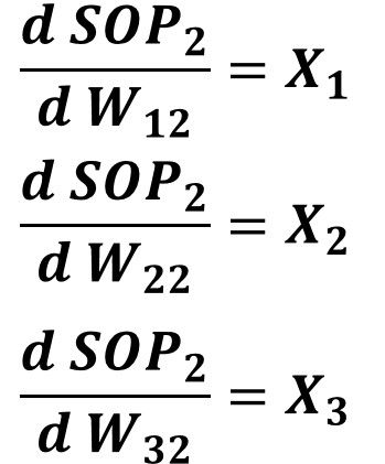
In order to update the weights W11, W21, and W31, the last derivative to calculate is the derivative between SOP1 to all of these weights. At first, we have to keep the equation relating SOP1 to all of these weights in mind. It is repeated below.

SOP1=X1*W11+X2*W21+X3*W31

The derivative of SOP1 to all of these 3 weights are given in the equations below.

Similarly, we have to keep the equation relating SOP2 to the weights W12, W22, and W32 in mind and this is why it is repeated again below.

SOP2=X1*W12+X2*W22+X3*W32

The derivatives of SOP2 to W12, W22, and W32 are given in the next figure.

After calculating all derivatives in the chain from the error to all weights between the input and hidden layers, next is to multiply them for calculating the gradient by which such weights will be updated.

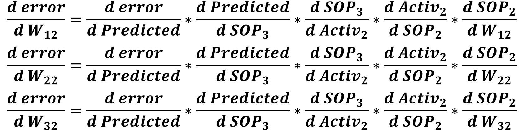
For the weights connected to the first hidden neuron which are W11, W21, and W31, their gradients will be calculated using the chains below. Note that all of these chains share all derivatives unless the last derivative.

For the weights connected to the second hidden neuron which are W12, W22, and W32, their gradients will be calculated using the chains below. Note that all of these chains share all derivatives unless the last derivative.

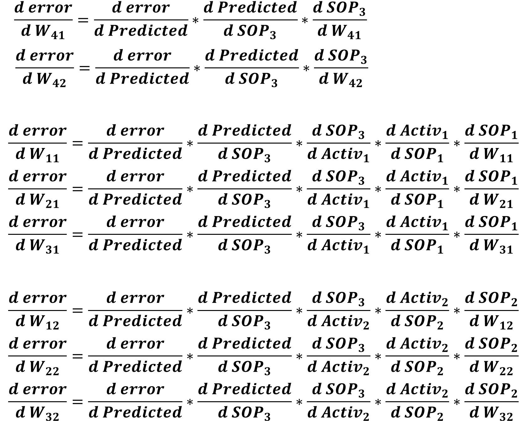
At that point, we have successfully prepared the chains for calculating the gradients for all weights in the entire network. We can summarize all of these chains in the next figure.

After understanding the theory behind implementing the GD algorithm for the current network, next is to start the Python implementation for such an algorithm. Note that the implementation is highly dependent on the implementation developed in the previous parts of this series.

Python Implementation

The complete code for implementing an ANN with 3 inputs, 1 hidden layer with 2 neurons, and 1 output neuron and optimizing it using the GD algorithm is listed below. The parts of this code will be discussed.

import numpy


def sigmoid(sop):
    return 1.0 / (1 + numpy.exp(-1 * sop))


def error(predicted, target):
    return numpy.power(predicted - target, 2)


def error_predicted_deriv(predicted, target):
    return 2 * (predicted - target)


def sigmoid_sop_deriv(sop):
    return sigmoid(sop) * (1.0 - sigmoid(sop))


def sop_w_deriv(x):
    return x


def update_w(w, grad, learning_rate):
    return w - learning_rate * grad


x = numpy.array([0.1, 0.4, 4.1])
target = numpy.array([0.2])

learning_rate = 0.001

w1_3 = numpy.random.rand(3)
w2_3 = numpy.random.rand(3)
w3_2 = numpy.random.rand(2)
w3_2_old = w3_2
print("Initial W : ", w1_3, w2_3, w3_2)

# Forward Pass
# Hidden Layer Calculations
sop1 = numpy.sum(w1_3 * x)
sop2 = numpy.sum(w2_3 * x)

sig1 = sigmoid(sop1)
sig2 = sigmoid(sop2)

# Output Layer Calculations
sop3 = numpy.sum(w3_2 * numpy.array([sig1, sig2]))

predicted = sigmoid(sop3)
err = error(predicted, target)

# Backward Pass
g1 = error_predicted_deriv(predicted, target)

### Working with weights between hidden and output layer
g2 = sigmoid_sop_deriv(sop3)

g3 = numpy.zeros(w3_2.shape[0])
g3[0] = sop_w_deriv(sig1)
g3[1] = sop_w_deriv(sig2)

grad_hidden_output = g3 * g2 * g1

w3_2 = update_w(w3_2, grad_hidden_output, learning_rate)

### Working with weights between input and hidden layer
# First Hidden Neuron
g3 = sop_w_deriv(w3_2_old[0])
g4 = sigmoid_sop_deriv(sop1)

g5 = sop_w_deriv(x)

grad_hidden1_input = g5 * g4 * g3 * g2 * g1

w1_3 = update_w(w1_3, grad_hidden1_input, learning_rate)

# Second Hidden Neuron
g3 = sop_w_deriv(w3_2_old[1])
g4 = sigmoid_sop_deriv(sop2)

g5 = sop_w_deriv(x)

grad_hidden2_input = g5 * g4 * g3 * g2 * g1

w2_3 = update_w(w2_3, grad_hidden2_input, learning_rate)

w3_2_old = w3_2
print(predicted)

At first, the inputs and the output are prepared using these 2 lines:

x = numpy.array([0.1, 0.4, 4.1])
target = numpy.array([0.2])

After that, the network weights are prepared according to these lines. Note that w1_3 is an array holding the 3 weights connecting the 3 inputs to the first hidden neuron. w2_3 is an array holding the 3 weights connecting the 3 inputs to the second hidden neuron. Finally, w3_2 is an array with 2 weights which are for the connections between the hidden layer neurons and the output neuron.

w1_3 = numpy.random.rand(3)
w2_3 = numpy.random.rand(3)
w3_2 = numpy.random.rand(2)

After preparing the inputs and the weights, next is to go through the forward pass according to the code below. It starts by calculating the sum of products for the 2 hidden neurons then feeding them to the sigmoid function. The 2 outputs of the sigmoid functions are multiplied by the 2 weights connected to the output neuron to return sop3. This is also applied as input to the sigmoid function to return the predicted output. Finally, the error is calculated.

# Forward Pass
# Hidden Layer Calculations
sop1 = numpy.sum(w1_3 * x)
sop2 = numpy.sum(w2_3 * x)

sig1 = sigmoid(sop1)
sig2 = sigmoid(sop2)

# Output Layer Calculations
sop3 = numpy.sum(w3_2 * numpy.array([sig1, sig2]))

predicted = sigmoid(sop3)
err = error(predicted, target)

After the forward pass is complete, next is to go through the backward pass. The part of the code responsible for updating the weights between the hidden and output layer is given below. The error to predicted output derivative is calculated and saved in the variable g1. g2holds the predicted output to SOP3 derivative. Finally, the SOP3 to W41 and W42 derivatives are calculated and saved in the variable g3. After calculating all derivatives required to calculate the gradients for W41 and W41, the gradients are calculated and saved in the grad_hidden_output variable. Finally, these weights are updated using the update_w() function by passing the old weights, gradients, and learning rate.

# Backward Pass
g1 = error_predicted_deriv(predicted, target)

### Working with weights between hidden and output layer
g2 = sigmoid_sop_deriv(sop3)

g3 = numpy.zeros(w3_2.shape[0])
g3[0] = sop_w_deriv(sig1)
g3[1] = sop_w_deriv(sig2)

grad_hidden_output = g3 * g2 * g1

w3_2 = update_w(w3_2, grad_hidden_output, learning_rate)

After updating the weights between the hidden and output layers, next is to work on the weights between the input and hidden layers. Here is the code required to update the weights connected to the first hidden neuron. g3 represents the SOP3 to Activ1 derivative. Because such derivative is calculated using the old values of the weights between the hidden and output layers, not the updated ones, then the old weights are saved into the w3_2_old variable for being used in this step. g4 represents the Activ1 to SOP1 derivative. Finally, g5 represents the SOP1to weights (W11, W21, and W31) derivatives.

When the gradients of such 3 weights are calculated, g3, g4, and g5 are multiplied by each other. They are also got multiplied by g2 and g1 calculated while updating the weights between the hidden and output layers. Based on the calculated gradients, the weights connecting the 3 inputs to the first hidden neuron are updated.

### Working with weights between input and hidden layer
# First Hidden Neuron
g3 = sop_w_deriv(w3_2_old[0])
g4 = sigmoid_sop_deriv(sop1)

g5 = sop_w_deriv(x)

grad_hidden1_input = g5*g4*g3*g2*g1

w1_3 = update_w(w1_3, grad_hidden1_input, learning_rate)

Similar to working on the 3 weights connected to the first hidden neuron, the other 3 weights connected to the second hidden neuron are updated according to the code below.

# Second Hidden Neuron
g3 = sop_w_deriv(w3_2_old[1])
g4 = sigmoid_sop_deriv(sop2)

g5 = sop_w_deriv(x)

grad_hidden2_input = g5*g4*g3*g2*g1

w2_3 = update_w(w2_3, grad_hidden2_input, learning_rate)

At the end of the code, the w3_2_old variable is set equal to w3_2.

w3_2_old = w3_2

By reaching this step, the entire code for implementing the GD algorithm for our example is now complete. The remaining edit is to use a loop for going through a number of iterations for updating the weights to make better predictions. Here is the updated code.

import numpy

def sigmoid(sop):
    return 1.0/(1+numpy.exp(-1*sop))

def error(predicted, target):
    return numpy.power(predicted-target, 2)

def error_predicted_deriv(predicted, target):
    return 2*(predicted-target)

def sigmoid_sop_deriv(sop):
    return sigmoid(sop)*(1.0-sigmoid(sop))

def sop_w_deriv(x):
    return x

def update_w(w, grad, learning_rate):
    return w - learning_rate*grad

x = numpy.array([0.1, 0.4, 4.1])
target = numpy.array([0.2])

learning_rate = 0.001

w1_3 = numpy.random.rand(3)
w2_3 = numpy.random.rand(3)
w3_2 = numpy.random.rand(2)
w3_2_old = w3_2
print("Initial W : ", w1_3, w2_3, w3_2)

for k in range(80000):
    # Forward Pass
    # Hidden Layer Calculations
    sop1 = numpy.sum(w1_3*x)
    sop2 = numpy.sum(w2_3*x)
    
    sig1 = sigmoid(sop1)
    sig2 = sigmoid(sop2)

    # Output Layer Calculations
    sop3 = numpy.sum(w3_2*numpy.array([sig1, sig2]))

    predicted = sigmoid(sop3)
    err = error(predicted, target)
    
    # Backward Pass
    g1 = error_predicted_deriv(predicted, target)

    ### Working with weights between hidden and output layer
    g2 = sigmoid_sop_deriv(sop3)

    g3 = numpy.zeros(w3_2.shape[0])
    g3[0] = sop_w_deriv(sig1)
    g3[1] = sop_w_deriv(sig2)
    
    grad_hidden_output = g3*g2*g1
    
    w3_2 = update_w(w3_2, grad_hidden_output, learning_rate)

    ### Working with weights between input and hidden layer
    # First Hidden Neuron
    g3 = sop_w_deriv(w3_2_old[0])
    g4 = sigmoid_sop_deriv(sop1)
    
    g5 = sop_w_deriv(x)

    grad_hidden1_input = g5*g4*g3*g2*g1
    
    w1_3 = update_w(w1_3, grad_hidden1_input, learning_rate)

    # Second Hidden Neuron
    g3 = sop_w_deriv(w3_2_old[1])
    g4 = sigmoid_sop_deriv(sop2)
    
    g5 = sop_w_deriv(x)

    grad_hidden2_input = g5*g4*g3*g2*g1
    
    w2_3 = update_w(w2_3, grad_hidden2_input, learning_rate)

    w3_2_old = w3_2
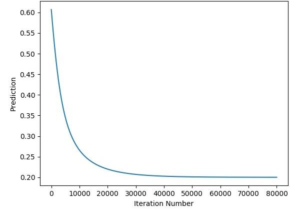
    print(predicted)

After the iterations complete, the next figure shows how the predicted output changes for the iterations.

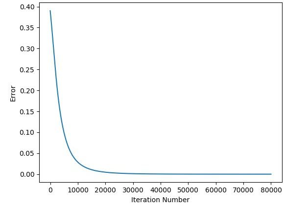
The next figure shows how the error changes for the iterations.

Working with 10 Inputs

The previous implementation used an input layer with just 3 inputs. What if more inputs are used? Is it required to do a lot of modifications to the code? The answer is NO because there are 2 minor modifications which are:

1. Editing the input array x for adding more inputs.
2. Editing the size of the weights arrays to return 10 weights rather than 3.

The implementation for working with 10 inputs is listed below. Everything in the code is identical to what was presented in the previous section except for the input array x which holds 10 values. Also, there are 10 weights returned using the numpy.random.rand() function. This is all you need to do.

import numpy


def sigmoid(sop):
    return 1.0 / (1 + numpy.exp(-1 * sop))


def error(predicted, target):
    return numpy.power(predicted - target, 2)


def error_predicted_deriv(predicted, target):
    return 2 * (predicted - target)


def sigmoid_sop_deriv(sop):
    return sigmoid(sop) * (1.0 - sigmoid(sop))


def sop_w_deriv(x):
    return x


def update_w(w, grad, learning_rate):
    return w - learning_rate * grad


x = numpy.array([0.1, 0.4, 4.1, 4.3, 1.8, 2.0, 0.01, 0.9, 3.8, 1.6])
target = numpy.array([0.2])

learning_rate = 0.001

w1_10 = numpy.random.rand(10)
w2_10 = numpy.random.rand(10)
w3_2 = numpy.random.rand(2)
w3_2_old = w3_2
print("Initial W : ", w1_10, w2_10, w3_2)

for k in range(80000):
    # Forward Pass
    # Hidden Layer Calculations
    sop1 = numpy.sum(w1_10 * x)
    sop2 = numpy.sum(w2_10 * x)

    sig1 = sigmoid(sop1)
    sig2 = sigmoid(sop2)

    # Output Layer Calculations
    sop3 = numpy.sum(w3_2 * numpy.array([sig1, sig2]))

    predicted = sigmoid(sop3)
    err = error(predicted, target)

    # Backward Pass
    g1 = error_predicted_deriv(predicted, target)

    ### Working with weights between hidden and output layer
    g2 = sigmoid_sop_deriv(sop3)

    g3 = numpy.zeros(w3_2.shape[0])
    g3[0] = sop_w_deriv(sig1)
    g3[1] = sop_w_deriv(sig2)

    grad_hidden_output = g3 * g2 * g1

    w3_2[0] = update_w(w3_2[0], grad_hidden_output[0], learning_rate)
    w3_2[1] = update_w(w3_2[1], grad_hidden_output[1], learning_rate)

    ### Working with weights between input and hidden layer
    # First Hidden Neuron
    g3 = sop_w_deriv(w3_2_old[0])
    g4 = sigmoid_sop_deriv(sop1)

    g5 = numpy.zeros(w1_10.shape[0])
    g5 = sop_w_deriv(x)

    grad_hidden1_input = g5 * g4 * g3 * g2 * g1

    w1_10 = update_w(w1_10, grad_hidden1_input, learning_rate)

    # Second Hidden Neuron
    g3 = sop_w_deriv(w3_2_old[1])
    g4 = sigmoid_sop_deriv(sop2)

    g5 = numpy.zeros(w2_10.shape[0])
    g5 = sop_w_deriv(x)

    grad_hidden2_input = g5 * g4 * g3 * g2 * g1

    w2_10 = update_w(w2_10, grad_hidden2_input, learning_rate)

    w3_2_old = w3_2
    print(predicted)