Yann LeCun, director of AI research at Facebook and Professor at NYU described Generative Adversarial Networks, GANs as the most interesting idea in Machine Learning in the last 10 years. Since the invention of GANs in 2014 by Ian Goodfellow, we’ve seen a ton of variants of these interesting neural networks from several research groups like NVIDIA and Facebook but we are going to look at one from a research group at UC Berkeley called the Cycle Consistent Adversarial Network. Before we dive into a Cycle Consistent Adversarial network, CycleGAN for short, we are going to look at what a Generative Adversarial Network is. This article is intended to give insights into the working mechanism of a Generative Adversarial Network and one of its popular variants, the Cycle Consistent Adversarial Network. Most of the code used here was taken from the official TensorFlow documentation page. Full code for this article can be obtained from : https://www.tensorflow.org/beta/tutorials/generative/cyclegan
Generative adversarial network
A Generative Adversarial Network is a type of neural network, normally consisting of two neural networks set up in an adversarial way. What I mean by adversarial way is that they work against each other in order to be better at what they do. These two networks are called the generator and discriminator. The first GAN was proposed by Ian Goodfellow in 2014 and after his work, we’ve seen several GANs, some with architectural novelty and others with improved performance and stability. So what exactly is a Generative Adversarial Network? In layman terms, A Generative Adversarial Network is a type of generative model consisting of two models where one model tries to generative images or some other real life data very close looking to the original real image or data to fool the other model while the other model optimizes itself by looking at the generated images and the authentic images in order not to get fooled by the generating model. In the literature of GANs, the model generating the images is called the generator and the model ensuring that the generator produces authentic looking images is called the discriminator. Let’s try to understand GANs using the detective-robber scenario. In this scenario, the robber acting as the generator continuously shows a counterfeit note of money to the detective who is acting as the discriminator. At each point in this process, the detective detects that the note is fake, rejects the money and informs the robber about what’s making the note fake. The robber also at each stage takes the note from the detective, uses the information from the detective to generate a new note note and then shows it again to the detective. This continues until the robber succeeds in creating a note that is authentic looking enough to fool the detective. That is exactly how a Generative Adversarial Network works - The generator produces synthetic images continuously and is optimized by receiving signal from the discriminator until the distribution of the synthetic images nearly matches the distribution of the original images.

A single training iteration step of a GAN involves three steps:
- first, the discriminator is shown a batch of real images and its weights optimized to classify these images as real images(real images labelled as 1)
- then we generate a batch of fake images using the generator, show these fake images to the discriminator and then optimize the weights of the discriminator to classify these images as fake images(fake images labelled as 0)
- the third step involves training the generator. We generate a batch of fake images, show these fake images to the discriminator but instead of optimizing the discriminator to classify these images as fake images, we optimize the generator to force the discriminator to classify these fakes images as real images.
Confused? Let’s break them down and you’ll see just how easy this is.
As mentioned earlier, first we show the discriminator a batch of real images and optimize it to classify these real images as real. Let assume that real images have 1 as their label and a simple absolute mean error is used as the loss function. Let’s also formulate the mathematical expression for the discriminator.We'll use f(x) where f(.) representing the discriminator is a feed forward neural network or Convolutional network and x is a real image or batch of real images. With the above parameters, our loss function should look something like this: | f(x) - 1 | (omitted the mean for simplicity). Feeding in a batch of real images and back-propagating this loss signal through the discriminator for optimization simply means that whenever our discriminator sees real images, we want it to predict a value really close to 1.The same process is used for step two but instead, we label the fake images generated by the generator as 0 so the loss function looks like this: | f(x)-0 | = | f(x) |. Back-propagating this loss signal through the discriminator and optimizing its weights means that whenever the discriminator is shown a fake image, we want it to predict a value very close to 0 which is the label of a fake image.Unlike steps one and two where we train the discriminator only, step three attempts to train the generator. We show the discriminator fakes images generated by the generator but this time we use the loss signature of step: | f(x) - 1 | . We then back-propagate the loss signal all the way from the discriminator to the generator and optimize the weights of the generator with this loss signal. This is synonymous to the discriminator informing the generator about the changes it needs to make in order to generate a fake image that will cause the discriminator to classify it as real.
Bring this project to life
You probably might be wondering how the generator produces the images. The originally proposed GAN generates images by taking in as input a fixed-size vector from a uniform distribution and gradually increasing the spatial dimension of this vector to form an image. Some recently invented GANs like the CycleGAN seem to have deviated from this generator architecture.

The task of image to image translation
Image to Image translation have been around for sometime before the invention of CycleGANs. One really interesting one is the work of Phillip Isola et al in the paper Image to Image Translation with Conditional Adversarial Networks where images from one domain are translated into images in another domain. The dataset for this work consists of aligned pair of images from each domain. This model was named Pix2Pix GAN.

The approach used by CycleGANs to perform Image to Image Translation is quite similar to Pix2Pix GAN with the exception of the fact that unpaired images are used for training CycleGANs and the objective function of the CycleGAN has an extra criterion, the cycle consistency loss. In fact both papers were written by almost the same authors.

As I mentioned earlier, some recent GANs have different Generator architectural design. Pix2Pix GANs and CycleGANs are major examples of GANs with this different architecture. Instead of taking in as input a fixed-size vector, it takes an image from one domain as input and outputs the corresponding image in the other domain. This architecture also makes use of skip connection to ensure that more features flow from input to output during forward propagation and gradients from loss to parameters during back-propagation. The discriminator architecture is almost the same. Unlike the initially proposed architecture which classifies a whole image as real or fake, the architecture used in these GANs classify patches of an image as real or fake by outputting a matrix of values as output instead of a single value. The reason for this is to encourage sharp high frequency detail and also to reduce the number of parameters.
Also, one major difference between the Pix2Pix GAN and the CycleGAN is that unlike the Pix2Pix GAN which consists of only two networks (Discriminator and Generator), the CycleGAN consists of four networks(two Discriminators and two Generators). Let’s look at objective function of a CycleGAN and how to train one.
The Objective Function
Earlier, I mentioned that there are three steps in training a GAN and that the first two steps trains the discriminator. Let’s look at how. We are going to combine the discriminator objective loss and implement it in one python function.
loss_obj = tf.keras.losses.BinaryCrossentropy(from_logits=True)

def discriminator_loss(real, generated):
  real_loss = loss_obj(tf.ones_like(real), real)

  generated_loss = loss_obj(tf.zeros_like(generated), generated)

  total_disc_loss = real_loss + generated_loss

  return total_disc_loss
Notice that instead of using a mean absolute error, we use a binary cross-entropy loss function. The real loss objective takes as input the discriminator output when a real image is fed into the discriminator and a matrix of ones. Recall that when we feed a real image into our discriminator, we want it to predict a value close to one so we are increasing this probability in this objective function. Same rule applies to the generated_loss - We are increasing the probability of the discriminator predicting a value close to zero when we feed in a fake image produced by the generator into the discriminator. We add both losses to back-propagate and train the discriminator. Next we train the generator.
def generator_loss(generated):
  return loss_obj(tf.ones_like(generated), generated)
We feed in fake images from the generator into the discriminator and instead of increasing the probability of the discriminator predicting a value close to one, we tweak the generator to force the discriminator to predict a value close to one. This is equivalent to back-propagating the gradients to the generator and updating its weights with the gradients. Let’s assume generator G maps images from domain X to Y and F maps images from domain Y to X. According to the paper, these adversarial losses only ensure that the learned mapping G and F produce outputs that match the distribution of Y and X respectively but are not visually identical to images in the respective domain. For instance, let’s assume we train G to map images from a domain containing images of summer scenes to a domain containing images of winter scenes. With only the adversarial losses used to learn the mapping, when we map an image x from the X domain using G, an image y is produced which only matches the distribution of Y and hence can be any random permutation of images in the Y domain which might not be identical to the input image, x. The mappings G and F are under-constrained mappings and to reduce the space of possible mappings, the authors introduced the cycle consistency loss to augment the adversarial loss. They theorized that to further constrain the mappings, the mappings should be cycle-consistent. This means that for each image x from the domain X, an image translation to the domain Y and back to the domain X should bring x back to the original image. that is x → G(x) → y → F(y) ≈ x. This is equivalent to x→G(x)→F(G(x)) ≈ x. They term this as forward cycle consistency. Similarly, for each image y from domain Y, G and F should satisfy the mapping y → F(y) → G(F(y)) ≈ y (backward cycle consistency).

    def calc_cycle_loss(real_image, cycled_image):
      loss1 = tf.reduce_mean(tf.abs(real_image - cycled_image))

      return LAMBDA * loss1
    #lambda is to provide weight to this objective function
We introduce a last loss function, the identity loss which further ensures that outputs from a mapping visually match the images from the domain they map to.

    def identity_loss(real_image, same_image):
      loss = tf.reduce_mean(tf.abs(real_image - same_image))
      return LAMBDA * 0.5 * loss
    #LAMBDA is to provide weight to this objective function
Models
In the paper for this work, the authors used a more refined architecture for their generator network. Its made up of skip connections similar to that in a Residual Network but we are going to use the Unet model implemented in the TensorFlow examples module. We can download and install module from https://github.com/tensorflow/examples or use:
!pip install git+https://github.com/tensorflow/examples.gitTo access models from the TensorFlow examples package, use the snippet:
from tensorflow_examples.models.pix2pix import pix2pix

generator_g = pix2pix.unet_generator(OUTPUT_CHANNELS, norm_type='instancenorm')
generator_f = pix2pix.unet_generator(OUTPUT_CHANNELS, norm_type='instancenorm')

discriminator_x = pix2pix.discriminator(norm_type='instancenorm', target=False)
discriminator_y = pix2pix.discriminator(norm_type='instancenorm', target=False)
The generator is made up of down-sampling and up-sampling layers. An input image is first passed through successive down-sampling layers which reduces the spatial dimension of the image or batch of images. Down-sampling is achieved by transpose convolutional layers. After sufficiently down-sampling the input image, we upsample it to increase it spatial dimension to form an image. Up-sampling is achieved by convolutional layers.
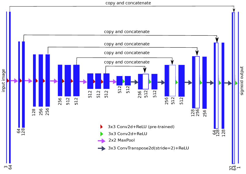
As already discussed, the discriminator network is a feed forward network, more specifically a convolutional neural network which outputs a matrix of values with each value representing the decision of discriminator on a patch or small region on the input image. So instead of classify an entire image as fake or real, it makes that decision on patches on the image.

we’ve already discussed the reason for this architecture.
Data
Obtaining data for Generative Adversarial Network can be quite of a challenge. Luckily for us, the TensorFlow dataset module consists of several dataset with unpaired alignment of images. You can install module using this simple command:
pip install tensorflow-datasetsAfter installing module, access dataset using the code below:
    dataset, metadata = tfds.load('cycle_gan/horse2zebra',
                                  with_info=True, as_supervised=True)

    train_X, train_Y = dataset['trainA'], dataset['trainB']
    test_X, test_Y = dataset['testA'], dataset['testB']
Notice that we are using a dataset with “horses” and “zebras” domains. There are a ton of other unpaired dataset here: https://www.tensorflow.org/datasets/catalog/cycle_gan - Just replace the “horse2zebra” in the load function with the dataset of your choice. Now that we have our dataset, we need to build an effective pipeline to feed the dataset into the neural networks. The tf.data API provides us with all the tools to create this pipeline.
    def random_crop(image):
      cropped_image = tf.image.random_crop(
          image, size=[IMG_HEIGHT, IMG_WIDTH, 3])
      return cropped_image

    # normalizing the images to [-1, 1]
    def normalize(image):
      image = tf.cast(image, tf.float32)
      image = (image / 127.5) - 1
      return image

    def random_jitter(image):
      # resizing to 286 x 286 x 3
      image = tf.image.resize(image, [286, 286],
                              method=tf.image.ResizeMethod.NEAREST_NEIGHBOR)
      # randomly cropping to 256 x 256 x 3
      image = random_crop(image)
      # random mirroring
      image = tf.image.random_flip_left_right(image)
      return image

    def preprocess_image_train(image, label):
      image = random_jitter(image)
      image = normalize(image)
      return image

    def preprocess_image_test(image, label):
      image = normalize(image)
      return image

    train_X = train_X .map(
        preprocess_image_train, num_parallel_calls=AUTOTUNE).cache().shuffle(
        BUFFER_SIZE).batch(1)

    train_Y = train_Y.map(
        preprocess_image_train, num_parallel_calls=AUTOTUNE).cache().shuffle(
        BUFFER_SIZE).batch(1)

    test_X = test_X.map(
        preprocess_image_test, num_parallel_calls=AUTOTUNE).cache().shuffle(
        BUFFER_SIZE).batch(1)

    test_Y = test_zebras.map(
        preprocess_image_test, num_parallel_calls=AUTOTUNE).cache().shuffle(
        BUFFER_SIZE).batch(1)
Basically what the above code does is to define a set of functions to manipulate images as they flow through the pipeline (data augmentation). We also batch the dataset and shuffle the images after each complete iteration through the dataset.
Throughout the article, we’ve talked about using adversarial and cycle consistent loss to train our models. Now we are going to see how to implement this training algorithm in code.
@tf.function
def train_step(real_x, real_y):
  # persistent is set to True because the tape is used more than
  # once to calculate the gradients.
  with tf.GradientTape(persistent=True) as tape:
    # Generator G translates X -> Y
    # Generator F translates Y -> X.

    fake_y = generator_g(real_x, training=True)
    cycled_x = generator_f(fake_y, training=True)

    fake_x = generator_f(real_y, training=True)
    cycled_y = generator_g(fake_x, training=True)

    # same_x and same_y are used for identity loss.
    same_x = generator_f(real_x, training=True)
    same_y = generator_g(real_y, training=True)

    disc_real_x = discriminator_x(real_x, training=True)
    disc_real_y = discriminator_y(real_y, training=True)

    disc_fake_x = discriminator_x(fake_x, training=True)
    disc_fake_y = discriminator_y(fake_y, training=True)

    disc_x_loss = discriminator_loss(disc_real_x, disc_fake_x)
    disc_y_loss = discriminator_loss(disc_real_y, disc_fake_y)

    # calculate the loss
    gen_g_loss = generator_loss(disc_fake_y)
    gen_f_loss = generator_loss(disc_fake_x)

    total_cycle_loss = calc_cycle_loss(real_x, cycled_x) + calc_cycle_loss(real_y, cycled_y)

    # Total generator loss = adversarial loss + cycle loss
    total_gen_g_loss = gen_g_loss + total_cycle_loss + identity_loss(real_y, same_y)
    total_gen_f_loss = gen_f_loss + total_cycle_loss + identity_loss(real_x, same_x)


  # Calculate the gradients for generator and discriminator
  generator_g_gradients = tape.gradient(total_gen_g_loss,
                                        generator_g.trainable_variables)
  generator_f_gradients = tape.gradient(total_gen_f_loss,
                                        generator_f.trainable_variables)

  discriminator_x_gradients = tape.gradient(disc_x_loss,
                                            discriminator_x.trainable_variables)
  discriminator_y_gradients = tape.gradient(disc_y_loss,
                                            discriminator_y.trainable_variables)

  # Apply the gradients to the optimizer
  generator_g_optimizer.apply_gradients(zip(generator_g_gradients,
                                            generator_g.trainable_variables))

  generator_f_optimizer.apply_gradients(zip(generator_f_gradients,
                                            generator_f.trainable_variables))

  discriminator_x_optimizer.apply_gradients(zip(discriminator_x_gradients,
                                                discriminator_x.trainable_variables))

  discriminator_y_optimizer.apply_gradients(zip(discriminator_y_gradients,
                                                discriminator_y.trainable_variables))
The tf.function decorator at the top of the train function compiles the entire train_step function into a TensorFlow graph to increase performance on hardware such as TPU and GPU. The train step function may be complicated but it follows the steps we described earlier in training a GAN. We first use the generators to produce the fakes images and cycle images. The fake images are used to train both the generator and the discriminator and the cycle images are used in the cycle consistent loss to ensure cycle consistency as we described earlier. In training the discriminator, we first feed in the real images into the discriminators to obtain the discriminator output for real images. We follow suit for the fake images produced by the generator to obtain the discriminator output for fake images. We then feed these outputs into the discriminator loss function and then train each discriminator using each discriminator's loss obtained. Now we move on to train the generators. We pass in the discriminators’ decision on fake images into the generator_loss function which describes how good the generators are in fooling the discriminators to think the images they produce are real images. We combine this loss with the cycle consistent loss and the identity loss which are both responsible at further constraining the possible mappings, obtain the gradients and optimize the weights of the generators. The train step function perform all these actions on a batch of images so we need to define a training loop to perform the train step iteratively on all batches of the dataset for some epochs. The training loop is made up of three stages.
- First we iterative through some number of epochs (integer value)
- And then at each epoch we iterative through the entire datasets consisting of batches of images (train_X and train_Y).
- Then for each batch of image we simply call the train_step function to train both the discriminators and generators on each batch of dataset.
The training loop also contain some if statements to log the statistics of our training on the screen.
for epoch in range(EPOCHS):
  start = time.time()

  n = 0
  for image_x, image_y in tf.data.Dataset.zip((train_horses, train_zebras)):
    train_step(image_x, image_y)
    if n % 10 == 0:
      print ('.', end='')
    n+=1

  clear_output(wait=True)
  # Using a consistent image (sample_horse) so that the progress of the model
  # is clearly visible.
  generate_images(generator_g, sample_horse)

  if (epoch + 1) % 5 == 0:
    ckpt_save_path = ckpt_manager.save()
    print ('Saving checkpoint for epoch {} at {}'.format(epoch+1,
                                                         ckpt_save_path))

  print ('Time taken for epoch {} is {} sec\n'.format(epoch + 1,
                                                      time.time()-start))
The generate_images function displays images generated by the generator. This is to keep track of how well our model is performing. Its implementation is shown below.
def generate_images(model, test_input):
prediction = model(test_input)
plt.figure(figsize=(12, 12))
display_list = [test_input[0], prediction[0]]
title = ['Input Image', 'Predicted Image']
for i in range(2):
plt.subplot(1, 2, i+1)
plt.title(title[i])
# getting the pixel values between [0, 1] to plot it.
plt.imshow(display_list[i] * 0.5 + 0.5)
plt.axis('off')
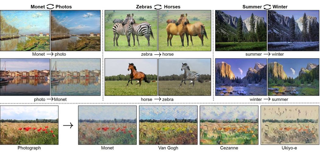
plt.show()Training takes some time so I suggest you perform the training on Paperspace gradient notebooks with GPU enabled environment to expedite the training process: Paperspace.com. After training models for a long time, the generators should be able to produce fairly realistic translated images like this:

Next steps
- There are several dataset with regards to the task of image to image translation in the TensorFlow dataset package. I entreat readers to try out different dataset and post their results on twitter. You can tag me @henryansah083
- We implemented the generators using the unet models. You should also experiment with other architectures such as the Residual Network Generator architecture proposed in the paper.
About me
I am an undergraduate student currently studying Electrical and Electronic Engineering. I am also a deep learning enthusiast and writer. My work mostly focuses on computer vision and natural language processing. I'm hoping to one day break into the field of autonomous vehicles.You can follow along on twitter(@henryansah083): https://twitter.com/henryansah083?s=09 LinkedIn: https://www.linkedin.com/in/henry-ansah-6a8b84167/.