In this tutorial we will implement the paper Continuous Control with Deep Reinforcement Learning, published by Google DeepMind and presented as a conference paper at ICRL 2016. The networks will be implemented in PyTorch using OpenAI gym. The algorithm combines Deep Learning and Reinforcement Learning techniques to deal with high-dimensional, i.e. continuous, action spaces.
After the success of Deep-Q Learning algorithm that led Google DeepMind to outperform humans in playing Atari games, they extended the same idea to physics tasks, where the action space is much bigger with respect to the one of the aforementioned games. Indeed, in a physics task, where the objective is generally to make a rigid-body learn a certain movement, the actions that can be applied to the actuators are continuous, i.e. they can span from a minimum to a maximum value within an interval.
One can simply ask: why don’t we discretize the action space?
Yes, we can, but consider a 3 degree-of-freedom system where each action, spanning within its own interval, is discretized into, let’s say, 10 values: the action space will have a dimensionality of 1000 (10^3) and this will lead to two big problems: the curse of dimensionality and an intractable approach for continuous control tasks, where a discretization of 10 samples for each action would not lead to a fine solution. Think about a robotic arm: an actuator doesn’t have just a few available values in terms of torque/force to be applied to produce velocities and accelerations for the rotation/translation operations.
Deep Q-Learning can deal well with high-dimensional state space (images as an input) but still it cannot deal with high dimensional action spaces (continuous action). A good example of Deep-Q Learning is the implementation of an AI that can play Dino Run, where the set of action space is simply: { jump, get_down, do_nothing}. The aforementioned tutorial is a good start if you want to know the basics of reinforcement learning and how to implement a Q-network, and I strongly suggest you go through it first if you are not familiar with reinforcement learning concepts.
What We Will Cover
In this tutorial we will go through the following steps:
- Explain the concept of policy network
- Combine Q-network and policy network in the so called actor-critic architecture
- See how the parameters are updated in order to maximize and minimize performance and objective functions
- Integrate memory buffer and freeze target network concepts, and understand what is the exploration strategy adopted in DDPG.
- Implement the algorithm using PyTorch: training on some of the OpenAI gym environment created for continuous control tasks, such as Pendulum and Mountain Car Continuous. More complex environments such as Hopper (to make a leg hop forward without falling) and the Double Inverted Pendulum (keep the pendulum in equilibrium by applying a force along the horizontal axis) require a MuJoCo license and you have to buy it or request it if you have an academic or institutional contact. Nonetheless, you can request a free 30-day license.
Getting Started With DDPG
As a general overview, the algorithm that is introduced in the paper is called Deep Deterministic Policy Gradient (DDPG). It continues from the previous successful DeepMind paper Playing Atari with Deep Reinforcement Learning with the concepts of Experience Replay Buffer, where the networks are trained off-policy by sampling experience batches, and Freeze Target Networks, where copies of the networks are made, with the purpose to be used in the objective functions to avoid divergence and instability of complex and non-linear function approximators such as neural networks.
Since the purpose of this tutorial is not to show the basics of reinforcement learning, if you are unfamiliar with these concepts I strongly suggest you first read the previously mentioned AI that can play Dino Run Paperspace tutorial. Once you are familiar with the concepts of Environment, Agent, Reward, and Q-value function (which is the function that in complex tasks is approximated by deep neural networks, hence called a Q-network) you are ready to dive into more sophisticated deep reinforcement learning architectures, like the Actor-Critic architecture that involves a combination of Policy network and Q-Network.
Reinforcement Learning In A Nutshell
Reinforcement Learning is a subfield of machine learning. It differs from the classic paradigms of supervised and unsupervised learning since it is a trial-and-error approach. This means that the agent is not actually trained on a dataset, but is instead trained by interacting with the environment, which is considered to be the entire system where we want the agent to act on (like a game, or a robotic arm). The clue point is that the environment must a provide a reward in response to the agent's actions. This reward is engineered depending on the task and must be well-thought since it is crucial for the entire progress of learning.
The basic elements of the trial-and-error procedure are the value functions, solved via Bellman equations in a discrete scenario, where we have both low-dimensional state and action spaces. When we deal with high-dimensional state space or action spaces we have to introduce complex and non-linear function approximators such as deep neural networks. For this reason, the concept of Deep Reinforcement Learning was introduced in the literature.
Let’s now start with a brief description of the main innovations brought by the DDPG for dealing with continuous, hence high-dimensional, action spaces in a Reinforcement Learning framework.
DDPG Building Blocks
Policy Network
Besides the usage of a neural network to parameterize the Q-function, as it happened with DQN, which is called the “critic” in the more sophisticated actor-critic architecture (the core of the DDPG), we have also the Policy network, called the “actor”. This neural network is then introduced to parameterize the policy function as well.
The policy is basically the agent behavior, a mapping from state to action (in case of deterministic policy) or a distribution of actions (in case of stochastic policy). These two kind of policies exist because they are suitable for certain tasks: a deterministic policy is well-suited for physics control problem, while a stochastic policy is a great option for solving games problem.
In this case the output of the policy network is a value that corresponds to the action to be taken on the environment.
Objective and Loss Functions
We have two networks, hence two set of parameters to update: the parameters of the policy network have to be updated in order to maximize the performance measure J defined in the policy gradient theorem; while the parameters of the critic network are updated in order to minimize the temporal difference loss L.
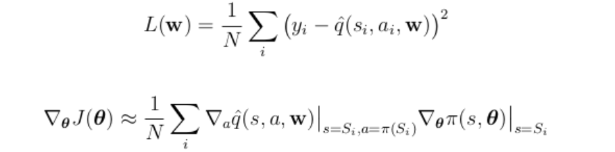
Basically, we need to improve the performance measure J in order to follow the maximization of the Q-value function, while minimizing the temporal difference loss as it happened with Deep Q-Network for playing Atari games.
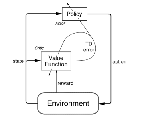
Actor-Critic architecture
Actor takes state as input to give action as output, while critic takes both state and action as input to give as output the value of the Q function. The critic uses gradient temporal-difference learning while the actor parameters are learned following policy gradient theorem. The main idea behind this architecture is that the policy network acts producing an action and the Q-network criticize that action.
Integrate experience replay and freeze target network
As with Q learning, the usage of non-linear function approximators like neural networks, which are necessary to generalize on large state spaces, means that convergence is no longer guaranteed. For this reason the usage of experience replay is needed in order to make independent and identically distributed samples. Moreover, frozen target networks need to be used in order to avoid divergence when updating the critic network. Differently from DQN, where the target network were updated every C steps, the parameters of the target networks are updated in DDPG case at every time step, following the "soft" update:
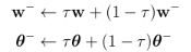
with τ << 1, w − and θ − respectively the weights of target Q-network and target policy network. With "soft" updates the weights of target networks are constrained to change slowly, thus improving the stability of learning and convergence results. The target network is then used in the temporal difference loss instead of the Q-network itself.
Exploration
The problem of exploration in algorithms like DDPG can be addressed in a very easy way and independently from the learning algorithm. Exploration policy is then constructed by adding noise sampled from a noise process N to the actor policy. The exploration policy thus becomes:
Where $\nu$ is an Ornstein-Uhlenbeck process, i.e. a stochastic process that can generate temporally correlated actions that guarantee smooth explorations in physical control problems.
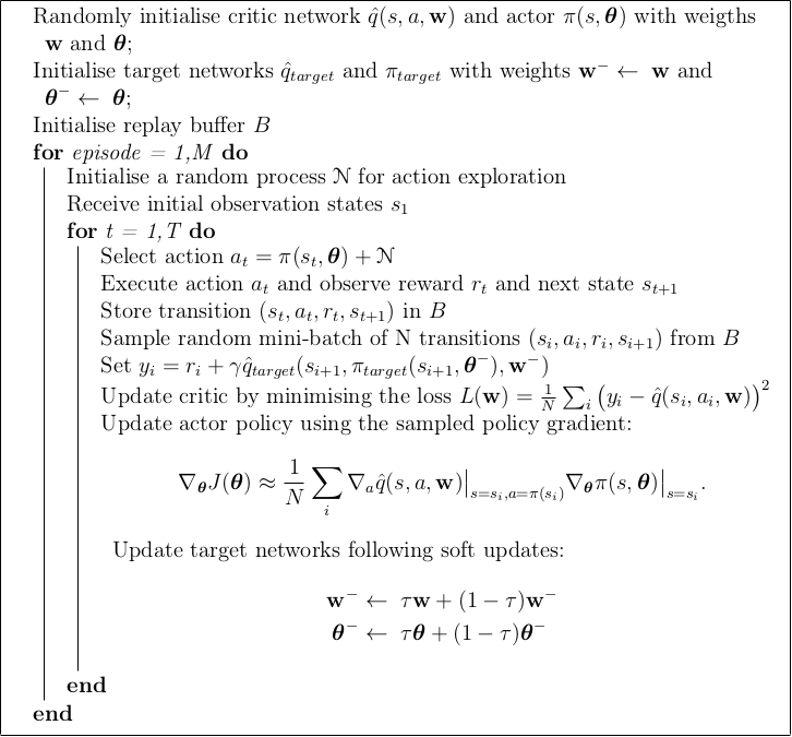
DDPG Algorithm: A Summary
Continuous control problems: an overview
We now have a look at the some of the environments that can be used to run the DDPG algorithm. These environments are available with gym package, and, as previously mentioned, some of them require MuJoCo (which is a physic engine) license to run. We are going to have a look at Pendulum environment, that does not require MuJoCo, and Hopper environment, which does.
Pendulum
Overview of the task
The purpose is to apply a torque on the central actuator to keep the pendulum in equilibrium on the vertical axis. This problem has a 3-dimensional state space, i.e. the cosine and sine of the angle as well as the derivative of the angle. The action space is 1-dimensional, which is the torque applied to the joint being bounded in the range $[-2, 2]$.
Reward function
The precise equation for reward:
-(theta^2 + 0.1*theta_dt^2 + 0.001*action^2)
Theta is normalized between -pi and pi. Therefore, the lowest cost is -(pi^2 + 0.1*8^2 + 0.001*2^2) = -16.2736044, and the highest cost is 0. In essence, the goal is to remain at zero angle (vertical), with the least rotational velocity, and the least effort.
For more details about Pendulum environment, check GitHub or OpenAI env page.
Hopper
The hopper task is to make a hopper with three joints and 4 body parts hop forward as fast as possible. It is available with gym but a MuJoCo license is needed, so you have to request it and install it for gym to work.
A general overview of the task
This problem has a 11 dimensional state vectors which includes: positions (in terms of radiant or meters if they are revolute or prismatic joints), derivatives of positions and both sin and cos functions of revolute joint angles with respect to their relative reference systems. The action space corresponds to a 3-dimensional space where each action is a continuous value that is bounded in the range $[−1, 1]$. So the network architecture shall have 3 output neurons with tanh activation function. These torques are applied on actuators that are found in the thigh joint, the leg joint and the foot joint, and the range for these actions is normalized to $[−1, 1]$.
Reward function
Since the objective of the task is to make the hopper move forward, the reward function is defined taking into account a bonus for being alive, a positive contribution of the forward velocity (computed by taking the derivative of the displacement at each step) and a negative contribution of the euclidean norm among the action control space.
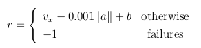
where a are the actions (i.e. the outputs of the network), vx is the forward velocity and b is a bonus for being alive. The episode terminates when at least one of the failure conditions occur, and they are:

where θ is the forward pitch of the body.
For more details about Hopper environment, check GitHub or OpenAI env page.
Other gym environments to play with
There are several gym environments that are suitable for continuous control since they have continuous action space. Some of them require MuJoCo, some do not.
Among the ones that do not require MuJoCo, you can try the code on Lunar Lander, Bipedal Walker or CarRacing. Notice that Car Racing has high dimensional state (image pixels), so you cannot use the fully connected layers used with low dimensional state space environment but an architecture that would include convolutional layers as well.
Code implementation
Setup
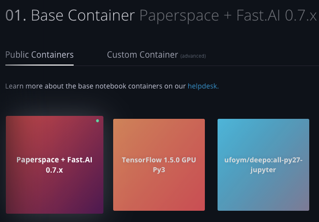
Set up the instance on Paperspace:
The public container "Paperspace + Fast.AI" is good to go with our experiment.
Configure: open a terminal and install Gym, upgrade torch version.
pip install gym
pip install --upgrade torch
The experiment will run on "Pendulum-v0" gym environment. Some environments needs MuJoCo license ("HalfCheetah-v1", "Hopper-v1", "Ant-v1" or "Humanoid-v1") while other needs PyBox2d to be run ("LunarLanderContinuous-v2", "CarRacing-v0" or "BipedalWalker-v2").
Once you have installed MuJoCo or PyBox2d for the environment that you want to play with ("Pendulum-v0" does not need any of these, just gym package), you can open a Jupyter Notebook and start coding.
General settings
The configuration follows the settings described in the supplementary information section of the DDPG paper, that you can find at page 11.
As described in the paper, we have to set a buffer size of 1 million entries, a batch size for sampling from memory equal to 64, a learning rate for actor and critic networks equal to 0.0001 and 0.001 respectively, a tau parameter for soft update equal to 0.001 and 300-400 neurons for the hidden layers of the networks.
BUFFER_SIZE=1000000
BATCH_SIZE=64  #this can be 128 for more complex tasks such as Hopper
GAMMA=0.9
TAU=0.001       #Target Network HyperParameters
LRA=0.0001      #LEARNING RATE ACTOR
LRC=0.001       #LEARNING RATE CRITIC
H1=400   #neurons of 1st layers
H2=300   #neurons of 2nd layers

MAX_EPISODES=50000 #number of episodes of the training
MAX_STEPS=200    #max steps to finish an episode. An episode breaks early if some break conditions are met (like too much
                  #amplitude of the joints angles or if a failure occurs)
buffer_start = 100
epsilon = 1
epsilon_decay = 1./100000 #this is ok for a simple task like inverted pendulum, but maybe this would be set to zero for more
                     #complex tasks like Hopper; epsilon is a decay for the exploration and noise applied to the action is
                     #weighted by this decay. In more complex tasks we need the exploration to not vanish so we set the decay
                     #to zero.
PRINT_EVERY = 10 #Print info about average reward every PRINT_EVERY

ENV_NAME = "Pendulum-v0" # For the hopper put "Hopper-v2"
#check other environments to play with at https://gym.openai.com/envs/
Experience Replay Buffer
It would be interesting to use prioritize experience replay. Have you ever managed to use the prioritized experience replay with DDPG? Leave a comment if you would like to share your results with prioritized experience replay.
Regardless, below there is the implementation of a simple replay buffer without priority.
from collections import deque
import random
import numpy as np

class replayBuffer(object):
    def __init__(self, buffer_size, name_buffer=''):
        self.buffer_size=buffer_size  #choose buffer size
        self.num_exp=0
        self.buffer=deque()

    def add(self, s, a, r, t, s2):
        experience=(s, a, r, t, s2)
        if self.num_exp < self.buffer_size:
            self.buffer.append(experience)
            self.num_exp +=1
        else:
            self.buffer.popleft()
            self.buffer.append(experience)

    def size(self):
        return self.buffer_size

    def count(self):
        return self.num_exp

    def sample(self, batch_size):
        if self.num_exp < batch_size:
            batch=random.sample(self.buffer, self.num_exp)
        else:
            batch=random.sample(self.buffer, batch_size)

        s, a, r, t, s2 = map(np.stack, zip(*batch))

        return s, a, r, t, s2

    def clear(self):
        self.buffer = deque()
        self.num_exp=0
Network architectures
We define here the networks. The structure follows the description of the paper: the actor is composed of three fully connected layers and has a hyperbolic tangent as output activation function, to deal with a [-1, 1] value range. The critic takes both state and action as input and outputs the Q-value after three fully connected layers.
def fanin_(size):
    fan_in = size[0]
    weight = 1./np.sqrt(fan_in)
    return torch.Tensor(size).uniform_(-weight, weight)

class Critic(nn.Module):
    def __init__(self, state_dim, action_dim, h1=H1, h2=H2, init_w=3e-3):
        super(Critic, self).__init__()

        self.linear1 = nn.Linear(state_dim, h1)
        self.linear1.weight.data = fanin_(self.linear1.weight.data.size())

        self.linear2 = nn.Linear(h1+action_dim, h2)
        self.linear2.weight.data = fanin_(self.linear2.weight.data.size())

        self.linear3 = nn.Linear(h2, 1)
        self.linear3.weight.data.uniform_(-init_w, init_w)

        self.relu = nn.ReLU()

    def forward(self, state, action):
        x = self.linear1(state)
        x = self.relu(x)
        x = self.linear2(torch.cat([x,action],1))

        x = self.relu(x)
        x = self.linear3(x)

        return x


class Actor(nn.Module):
    def __init__(self, state_dim, action_dim, h1=H1, h2=H2, init_w=0.003):
        super(Actor, self).__init__()
        self.linear1 = nn.Linear(state_dim, h1)
        self.linear1.weight.data = fanin_(self.linear1.weight.data.size())


        self.linear2 = nn.Linear(h1, h2)
        self.linear2.weight.data = fanin_(self.linear2.weight.data.size())

        self.linear3 = nn.Linear(h2, action_dim)
        self.linear3.weight.data.uniform_(-init_w, init_w)

        self.relu = nn.ReLU()
        self.tanh = nn.Tanh()

    def forward(self, state):
        x = self.linear1(state)
        x = self.relu(x)
        x = self.linear2(x)
        x = self.relu(x)
        x = self.linear3(x)
        x = self.tanh(x)
        return x

    def get_action(self, state):
        state  = torch.FloatTensor(state).unsqueeze(0).to(device)
        action = self.forward(state)
        return action.detach().cpu().numpy()[0]
Exploration
As described in the paper, we have to add noise to the action in order to ensure exploration. An Ornstein-Uhlenbeck process is chosen because it adds noise in a smooth way, which is suitable for continuous control tasks. More details on this random process are simply described on Wikipedia.
# Based on http://math.stackexchange.com/questions/1287634/implementing-ornstein-uhlenbeck-in-matlab
class OrnsteinUhlenbeckActionNoise:
    def __init__(self, mu=0, sigma=0.2, theta=.15, dt=1e-2, x0=None):
        self.theta = theta
        self.mu = mu
        self.sigma = sigma
        self.dt = dt
        self.x0 = x0
        self.reset()

    def __call__(self):
        x = self.x_prev + self.theta * (self.mu - self.x_prev) * self.dt + self.sigma * np.sqrt(self.dt) * np.random.normal(size=self.mu.shape)
        self.x_prev = x
        return x

    def reset(self):
        self.x_prev = self.x0 if self.x0 is not None else np.zeros_like(self.mu)

    def __repr__(self):
        return 'OrnsteinUhlenbeckActionNoise(mu={}, sigma={})'.format(self.mu, self.sigma)
Setup training
We set up the training by initializing the environment, the networks, the target networks, the replay memory and the optimizers.
torch.manual_seed(-1)

env = NormalizedEnv(gym.make(ENV_NAME))

state_dim = env.observation_space.shape[0]
action_dim = env.action_space.shape[0]

print("State dim: {}, Action dim: {}".format(state_dim, action_dim))


noise = OrnsteinUhlenbeckActionNoise(mu=np.zeros(action_dim))

critic  = Critic(state_dim, action_dim).to(device)
actor = Actor(state_dim, action_dim).to(device)

target_critic  = Critic(state_dim, action_dim).to(device)
target_actor = Actor(state_dim, action_dim).to(device)

for target_param, param in zip(target_critic.parameters(), critic.parameters()):
    target_param.data.copy_(param.data)

for target_param, param in zip(target_actor.parameters(), actor.parameters()):
    target_param.data.copy_(param.data)


q_optimizer  = opt.Adam(critic.parameters(),  lr=LRC)
policy_optimizer = opt.Adam(actor.parameters(), lr=LRA)

MSE = nn.MSELoss()

memory = replayBuffer(BUFFER_SIZE)
writer = SummaryWriter() #initialise tensorboard writer
Iterate through episodes
MAX_EPISODES and MAX_STEPS parameters can be tuned according to the kind of the environment on which we are going to train the agent. In the case of a simple pendulum we do not have a failure condition for each episode so it will always go through the max steps for each episode; in a task where there is a failure condition, an agent will not go through all the steps (at least at the beginning, when it has not yet learned how to accomplish the task).
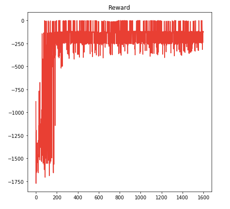
plot_reward = []
plot_policy = []
plot_q = []
plot_steps = []


best_reward = -np.inf
saved_reward = -np.inf
saved_ep = 0
average_reward = 0
global_step = 0
#s = deepcopy(env.reset())

for episode in range(MAX_EPISODES):
    #print(episode)
    s = deepcopy(env.reset())
    #noise.reset()

    ep_reward = 0.
    ep_q_value = 0.
    step=0

    for step in range(MAX_STEPS):
        #loss=0
        global_step +=1
        epsilon -= epsilon_decay
        #actor.eval()
        a = actor.get_action(s)
        #actor.train()

        a += noise()*max(0, epsilon)
        a = np.clip(a, -1., 1.)
        s2, reward, terminal, info = env.step(a)


        memory.add(s, a, reward, terminal,s2)

        #keep adding experiences to the memory until there are at least minibatch size samples

        if memory.count() > buffer_start:
            s_batch, a_batch, r_batch, t_batch, s2_batch = memory.sample(BATCH_SIZE)

            s_batch = torch.FloatTensor(s_batch).to(device)
            a_batch = torch.FloatTensor(a_batch).to(device)
            r_batch = torch.FloatTensor(r_batch).unsqueeze(1).to(device)
            t_batch = torch.FloatTensor(np.float32(t_batch)).unsqueeze(1).to(device)
            s2_batch = torch.FloatTensor(s2_batch).to(device)


            #compute loss for critic
            a2_batch = target_actor(s2_batch)
            target_q = target_critic(s2_batch, a2_batch)
            y = r_batch + (1.0 - t_batch) * GAMMA * target_q.detach() #detach to avoid backprop target
            q = critic(s_batch, a_batch)

            q_optimizer.zero_grad()
            q_loss = MSE(q, y)
            q_loss.backward()
            q_optimizer.step()

            #compute loss for actor
            policy_optimizer.zero_grad()
            policy_loss = -critic(s_batch, actor(s_batch))
            policy_loss = policy_loss.mean()
            policy_loss.backward()
            policy_optimizer.step()

            #soft update of the frozen target networks
            for target_param, param in zip(target_critic.parameters(), critic.parameters()):
                target_param.data.copy_(
                    target_param.data * (1.0 - TAU) + param.data * TAU
                )

            for target_param, param in zip(target_actor.parameters(), actor.parameters()):
                target_param.data.copy_(
                    target_param.data * (1.0 - TAU) + param.data * TAU
                )

        s = deepcopy(s2)
        ep_reward += reward


        #if terminal:
        #    noise.reset()
        #    break

    try:
        plot_reward.append([ep_reward, episode+1])
        plot_policy.append([policy_loss.data, episode+1])
        plot_q.append([q_loss.data, episode+1])
        plot_steps.append([step+1, episode+1])
    except:
        continue
    average_reward += ep_reward

    if ep_reward > best_reward:
        torch.save(actor.state_dict(), 'best_model_pendulum.pkl') #Save the actor model for future testing
        best_reward = ep_reward
        saved_reward = ep_reward
        saved_ep = episode+1

    if (episode % PRINT_EVERY) == (PRINT_EVERY-1):    # print every print_every episodes
        subplot(plot_reward, plot_policy, plot_q, plot_steps)
        print('[%6d episode, %8d total steps] average reward for past {} iterations: %.3f'.format(PRINT_EVERY) %
              (episode + 1, global_step, average_reward / PRINT_EVERY))
        print("Last model saved with reward: {:.2f}, at episode {}.".format(saved_reward, saved_ep))
        average_reward = 0 #reset average reward
Conclusions
The code snippets in this tutorial are a part of a more complete notebook that you may find on GitHub at this link. The networks used in that notebook are suitable for low-dimensional state space; if you want to deal with image inputs you have to add convolutional layers, as described at page 11 of the research paper.
Feel free to share your experience with other environments or approaches to improve the overall training process!