Implementation of Denoising Diffusion Probabilistic Model using Pytorch

In this tutorial, we show how to implement DDPMs in a GPU powered Paperspace Notebook to train a custom diffusion model on any image set.

8 months ago • 5 min read

By Adrien Payong

Introduction

Diffusion-based generative models were first presented in the year 2015, and Ho et al.'s publication of the work titled "Denoising Diffusion Probabilistic Models" (DDPMs) in the year 2020 was the catalyst that led to their widespread adoption . An interesting field of study known as diffusion probabilistic modeling is showing a lot of promise in the field of image generation. The idea behind diffusion models is to break the process of image generation into a sequential application of denoising autoencoders. This is the fundamental concept underlying these models. The method of reverse diffusion is then used to carry out the "denoising" operation in an iterative manner, taking place in a series of small steps that bring us back to the data subspace.

Denoising Diffusion Probabilistic Model and how does it work

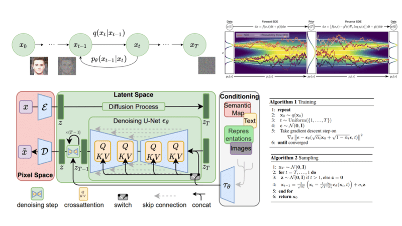
The Denoising Diffusion Probabilistic Model, often known as the DDPM, is an example of a generative model. Its purpose is to produce new images that are very similar to an original collection of images by using denoising techniques. The DDPM will operate as described below:

Using a technique called forward diffusion, DDPM gradually introduces Gaussian noise into the original image.
Over time, the variance of the Gaussian noise decreases, resulting in a less noisy image.
The DDPM uses a neural network to predict the amount of noise introduced to the image at each step of the forward diffusion process.
The DDPM uses the predicted noise in what is referred to as the "reverse process," which is a sequence of steps used to eliminate the noise from the image.
A new image is generated through the reverse process that is very similar to the original, but has less noise.
Using a maximum likelihood estimate technique, the DDPM is trained to make predictions about the noise introduced at each step of the forward diffusion process.

Implementation with Pytorch

Installation

If you're using PyTorch, you can get the denoising_diffusion_pytorch package to install the denoising diffusion model.

$ pip install denoising_diffusion_pytorch

Usage

The below code snippet shows how to implement the denoising diffusion model in PyTorch.

import torch
from denoising_diffusion_pytorch import Unet, GaussianDiffusion

model = Unet(
    dim = 64,
    dim_mults = (1, 2, 4, 8)
)

diffusion = GaussianDiffusion(
    model,
    image_size = 128,
    timesteps = 1000    # number of steps
)

training_images = torch.rand(8, 3, 128, 128) # images are normalized from 0 to 1
loss = diffusion(training_images)
loss.backward()
# after a lot of training

sampled_images = diffusion.sample(batch_size = 4)
sampled_images.shape # (4, 3, 128, 128)

The above code makes use of the denoising_diffusion_pytorch package's Unet and GaussianDiffusion classes.
The GaussianDiffusion class describes the diffusion model by using the denoising model along with additional parameters such as image size and number of timesteps. The Unet model defined by this code has a 64-level depth and a downsampling factor of (1, 2, 4, 8).
The training_images variable is a tensor that contains eight noisy images. The training_images tensor is sent as input to the diffusion object, which is then used to denoise the image.
The denoising loss that was determined by the diffusion model is the variable that represents the loss.
To calculate the loss gradients with respect to the model parameters, we use the backward() function on the loss variable.
The sampled_images variable is a tensor containing 4 denoised images produced by the diffusion model through the sample() function.

Alternately, the Trainer class allows for straightforward model training by the simple input of a folder name and the desired image dimensions.

from denoising_diffusion_pytorch import Unet, GaussianDiffusion, Trainer

model = Unet(
    dim = 64,
    dim_mults = (1, 2, 4, 8)
)

diffusion = GaussianDiffusion(
    model,
    image_size = 128,
    timesteps = 1000,           # number of steps
    sampling_timesteps = 250    # number of sampling timesteps (using ddim for faster inference [see citation for ddim paper])
)

trainer = Trainer(
    diffusion,
    'path/to/your/images',
    train_batch_size = 32,
    train_lr = 8e-5,
    train_num_steps = 700000,         # total training steps
    gradient_accumulate_every = 2,    # gradient accumulation steps
    ema_decay = 0.995,                # exponential moving average decay
    amp = True,                       # turn on mixed precision
    calculate_fid = True              # whether to calculate fid during training
)

trainer.train()

The Trainer class is where all of the training-specific settings are configured. This includes the diffusion object, the path to the training images, the batch size, the learning rate, the number of training steps, the gradient accumulation steps, the exponential moving average decay, the mixed-precision toggle, and the Fréchet Inception Distance (FID) calculation toggle.
To train the model, we use the train method on the trainer object.
Keep in mind that you'll need to change the path/to/your/images option to point to the location of the training images directory.
The number of data batches that are processed before the gradients are accumulated and the model parameters are updated is set by the gradient_accumulate_every parameter in the Trainer class of the denoising_diffusion_pytorch package.
During the training process, the exponential moving average (EMA) of the model parameters is given a decay rate that is specified by the ema_decay=0.995 parameter in the Trainer class of the denoising_diffusion_pytorch package.
Samples generated by Generative Adversarial Networks (GANs) and other generative models are often analyzed using the FID(Fréchet Inception Distance). The FID is a metric for gauging the degree to which real-world image distributions and synthetically-generated image distributions are similar in feature space. Generated images with a lower FID score are more likely to closely resemble the originals, indicating that the generative model is more accurate.

Conclusion

Overall, the DDPM is a robust generative model that may provide excellent results when used to generate new images. The model generates a new image that resembles the original but with less noise by first adding noise to the original image and then eliminating the noise. The model is then trained to provide maximum likelihood estimations of the noise levels at each step of the forward diffusion process. The DDPM has been used in a number of contexts due to its successful production of high-quality images without the need for adversarial training.