SCNet (CVPR 2020)

While attention methods in computer vision have had a fair share of the spotlight over the recent years, they have been strictly confined to the ways these methods are integrated into common convolutional neural networks (CNNs). Mostly these methods are used as plug-in modules which can be inserted into the structure of the different type of CNNs. However, in this blog post, we will take a look at a CVPR 2020 paper titled Improving Convolutional Networks with Self-Calibrated Convolutions by Liu. et. al., which proposes a new form of convolution operation called Self-calibrating convolution (SC-Conv) which has self-calibrating properties much similar to that of attention mechanisms.

First, we will take a look at the motivation behind the paper followed by certain subtle comparisons to GhostNet (CVPR 2020). We will then do a study of the structure of SC-Conv and will provide the PyTorch code for the same before concluding the post with the results and some critical comments.

Table of Contents

1. Motivation
2. Self Calibrating Convolution
3. Code
4. Results
5. Conclusion
6. References

Abstract

Recent advances on CNNs are mostly devoted to designing more complex architectures to enhance their representation learning capacity. In this paper, we consider improving the basic convolutional feature transformation process of CNNs without tuning the model architectures. To this end, we present a novel self-calibrated convolution that explicitly expands fields-of-view of each convolutional layer through internal communications and hence enriches the output features. In particular, unlike the standard convolutions that fuse spatial and channel-wise information using small kernels (e.g., 3 × 3), our self-calibrated convolution adaptively builds long-range spatial and inter-channel dependencies around each spatial location through a novel self-calibration operation. Thus, it can help CNNs generate more discriminative representations by explicitly incorporating richer information. Our self calibrated convolution design is simple and generic, and can be easily applied to augment standard convolutional layers without introducing extra parameters and complexity. Extensive experiments demonstrate that when applying our self-calibrated convolution into different backbones, the baseline models can be significantly improved in a variety of vision tasks, including image recognition, object detection, instance segmentation, and keypoint detection, with no need to change network architectures. We hope this work could provide future research with a promising way of designing novel convolutional feature transformation for improving convolutional networks.

Motivation

While a majority of research direction has been towards manually designing architectures or components like attention mechanisms or non-local blocks which enrich the feature representations of classic convolutional neural networks, this is sub-optimal and is very iterative.

In this paper, rather than designing complex network architectures to strengthen feature representations, we introduce self-calibrated convolution as an efficient way to help convolutional networks learn discriminative representations by augmenting the basic convolutional transformation per layer. Similar to grouped convolutions, it separates the convolutional filters of a specific layer into multiple portions but unevenly, the filters within each portion are leveraged in a heterogeneous way. Specifically, instead of performing all the convolutions over the input in the original space homogeneously, Self-calibrated convolutions transform the inputs to low-dimensional embeddings through down-sampling at first. The low-dimensional embeddings transformed by one filter portion are adopted to calibrate the convolutional transformations of the filters within another portion. Benefiting from such heterogeneous convolutions and between-filter communication, the receptive field for each spatial location can be effectively enlarged.

As an augmented version of the standard convolution, our self-calibrated convolution offers two advantages. First, it enables each spatial location to adaptively encode informative context from a long-range region, breaking the tradition of convolution operating within small regions (e.g., 3× 3). This makes the feature representations produced by our self-calibrated convolution more discriminative. Second, the proposed self-calibrated convolution is generic and can be easily applied to standard convolutional layers without introducing any parameters and complexity overhead or changing the hyper-parameters.

Self-Calibrating Convolutions

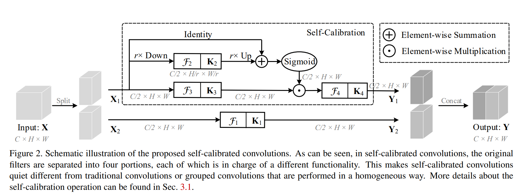
The above schematic illustration demonstrates the structural design of Self-Calibrating Convolutions (SC-Conv). At first glance, the structure seems to be a crossover of Ghost Convolution (CVPR 2020) and a conventional attention mechanism. Before we dive into SCConv, let's do a quick detour of GhostNet.

GhostNet (CVPR 2020)

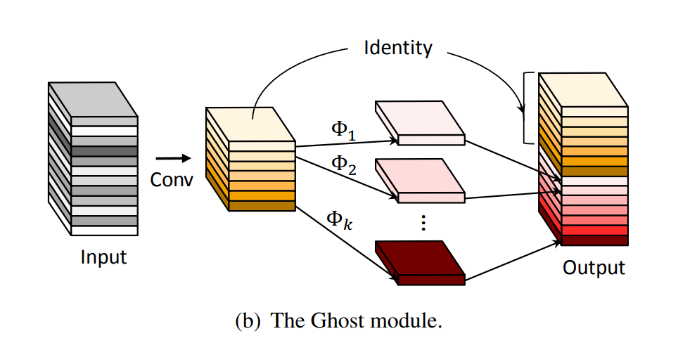
Published at CVPR 2020, GhostNet offered a simple way of reducing the parametric and computational complexity of large convolutional neural networks by replacing the standard convolution layers with a ghost layer. For a given input $X \in \mathbb{R}^{C \ast H \ast W}$ and an expected output of $\tilde{X} \in \mathbb{R}^{\hat{C} \ast H \ast W}$, ghost layer first generates $\frac{\hat{C}}{2}$ channels using standard convolution. Then the remaining $\frac{\hat{C}}{2}$ channels are generated by passing the first set of channels through a depthwise convolution kernel which essentially reduces parametric complexity by nearly half. For a more in-depth insight into GhostNet, please do read my post on the same here.

Alright, now back to SC Conv, there are two different branches in SC-Conv, one is the identity branch similar to an inherent residual branch while the other branch is responsible for self-calibration. Given an input tensor $X \in \mathbb{R}^{C \ast H \ast W}$ and an expected output tensor of the same shape $\hat{X}$, the tensor is first divided into two sets of each $\frac{C}{2}$ channels with the first branch simply applying a 2D convolution operation on one of the set. In the second branch, the set is passed through three parallel operations. The first operation is a simple channel preserving 2D convolution while in the second operation the spatial dimensions are downsampled by a factor of $r$ and then a 2D convolution is applied on the same, the output of which is subsequently upsampled by a factor of $r$ to preserve the same shape. The final operation is an identity function that is element-wise added to the upsampled feature maps from the second operation. The resultant tensor is passed through a sigmoid activation and then element-wise multiplied with the tensor obtained from the first tensor. Finally, this tensor is passed through yet another channel preserving 2D convolution. The two tensors from the two branches are then concatenated to form the complete set.

Code

import torch
import torch.nn as nn
import torch.nn.functional as F

class SCConv(nn.Module):
    def __init__(self, inplanes, planes, stride, padding, dilation, groups, pooling_r, norm_layer):
        super(SCConv, self).__init__()
        self.k2 = nn.Sequential(
                    nn.AvgPool2d(kernel_size=pooling_r, stride=pooling_r), 
                    nn.Conv2d(inplanes, planes, kernel_size=3, stride=1,
                                padding=padding, dilation=dilation,
                                groups=groups, bias=False),
                    norm_layer(planes),
                    )
        self.k3 = nn.Sequential(
                    nn.Conv2d(inplanes, planes, kernel_size=3, stride=1,
                                padding=padding, dilation=dilation,
                                groups=groups, bias=False),
                    norm_layer(planes),
                    )
        self.k4 = nn.Sequential(
                    nn.Conv2d(inplanes, planes, kernel_size=3, stride=stride,
                                padding=padding, dilation=dilation,
                                groups=groups, bias=False),
                    norm_layer(planes),
                    )

    def forward(self, x):
        identity = x

        out = torch.sigmoid(torch.add(identity, F.interpolate(self.k2(x), identity.size()[2:]))) # sigmoid(identity + k2)
        out = torch.mul(self.k3(x), out) # k3 * sigmoid(identity + k2)
        out = self.k4(out) # k4

        return out

You would require to download ImageNet dataset for training SCNet. You can download the same following the instructions here. Once downloaded you can train ImageNet using the following command in the jupyter environment linked above in paperspace gradient.

usage: train_imagenet.py  [-h] [-j N] [--epochs N] [--start-epoch N] [-b N]
                          [--lr LR] [--momentum M] [--weight-decay W] [--print-freq N]
                          [--resume PATH] [-e] [--pretrained] [--world-size WORLD_SIZE]
                          [--rank RANK] [--dist-url DIST_URL]
                          [--dist-backend DIST_BACKEND] [--seed SEED] [--gpu GPU]
                          [--multiprocessing-distributed]
                          DIR

PyTorch ImageNet Training

positional arguments:
  DIR                   path to dataset

optional arguments:
  -h, --help            show this help message and exit
  -j N, --workers N     number of data loading workers (default: 4)
  --epochs N            number of total epochs to run
  --start-epoch N       manual epoch number (useful on restarts)
  -b N, --batch-size N  mini-batch size (default: 256), this is the total
                        batch size of all GPUs on the current node when using
                        Data Parallel or Distributed Data Parallel
  --lr LR, --learning-rate LR
                        initial learning rate
  --momentum M          momentum
  --weight-decay W, --wd W
                        weight decay (default: 1e-4)
  --print-freq N, -p N  print frequency (default: 10)
  --resume PATH         path to latest checkpoint (default: none)
  -e, --evaluate        evaluate model on validation set
  --pretrained          use pre-trained model
  --world-size WORLD_SIZE
                        number of nodes for distributed training
  --rank RANK           node rank for distributed training
  --dist-url DIST_URL   url used to set up distributed training
  --dist-backend DIST_BACKEND
                        distributed backend
  --seed SEED           seed for initializing training.
  --gpu GPU             GPU id to use.
  --multiprocessing-distributed
                        Use multi-processing distributed training to launch N
                        processes per node, which has N GPUs. This is the
                        fastest way to use PyTorch for either single node or
                        multi node data parallel training

Note: You would require a Weights & Biases account to enable WandB Dashboard logging.

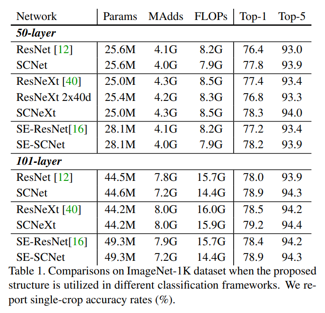
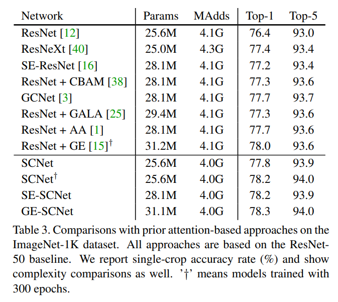
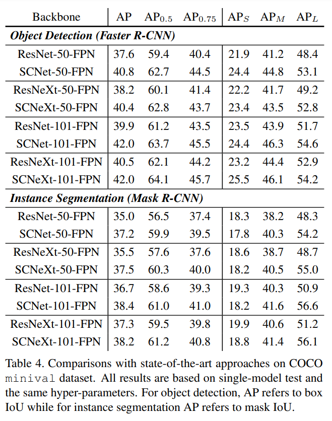
Results

Following are some of the results of SCNets as showcased in the paper:

Conclusion

SCNet offers a new approach of embedding attention mechanisms in convolutional neural networks unlike conventional attention mechanisms which are applied as an add-on module, SCConv can be used to replace conventional convolution layers. Although the approach ticks all the checkboxes of being cheap in terms of parameter/ FLOPs and offers a good performance boost, the only issue is of the added number of operations causes an increase in run-time.

References

1. Improving Convolutional Networks with Self-Calibrated Convolutions
2. SCConv official GitHub repository