In the first part of this series, we covered most of the essential theory and concepts related to transfer learning. We learned about convolutional neural networks, how they're used with transfer learning, and gained an understanding of fine-tuning these models. Finally, we also analyzed a few models popularly used for transfer learning. I would highly recommend checking out this Complete Intuitive Guide To Transfer Learning if you are new to this concept before proceeding further in this article.
In this article, we will focus on the practical aspects of transfer learning. We will cover an entire face recognition project with three different models, namely Resnet50, InceptionV3, and MobileNetV2. Feel free to experiment and try out new stuff to achieve better results. Please refer to the table of contents for the material that will be covered in this particular part of the article. Since this project is built from scratch, it is preferable to follow all of the contents accordingly.
You can run the full code for this article on a free GPU from a Gradient Community Notebook.
Table of Contents
- Introduction
- General tips and suggestions
- Data collection
- Data preparation (pre-processing the data)
- Data augmentation
1. Importing the required libraries
2. Setting the parameters
3. Augmentation of training and validation data - Model and architecture constructions
1. Assigning the different transfer learning architectures
2. Building the respective models - Callbacks, model compilation, and training
1. Defining the respective callbacks
2. Compilation of the models
3. Fitting the transfer learning models - Model prediction
1. Importing the libraries
2. Making the predictions - Conclusion
Bring this project to life
Introduction
While transfer learning models have tons of use cases in real-world applications, we will focus specifically on a face recognition project. With the help of this project, we can understand how several different types of models will work.
The primary objective of this article is to get you started with the use of transfer learning models on a fairly popular sample project. The overall performance of each model may not be as perfect as expected because of various parameters, constraints, data, and lesser epochs of training. However, it is only an example to show how you can build similar architectures and perform numerous projects with the help of these transfer learning models to achieve far better results on your own particular task.
General Tips and Suggestions
A few noteworthy tips and suggestions to keep in mind for the rest of the article is that we can always improve the quality of the models with further experimentation. The different models used here, namely ResNet50, InceptionV3, and MobileNetV2, are implemented to understand the logic behind a transfer learning project. However, any model may be better suited to one task than another, and these models may not be the best for every scenario. We will understand this point further as we explore and build out our project.
There are several advanced face recognition models that have been developed throughout the years. It is highly encouraged that various methods of improving the models such as fine-tuning, manipulating the different parameters, etc. be used as well. Changing even a small parameter or adding something like batch normalization or dropout can influence the model performance significantly.
Data collection
The first step in any machine learning or deep learning project involves getting your data in order. The collection of data for this particular face recognition task can be mainly done in two ways: by using an online dataset, or by creating your own custom dataset that will contain a few images of yourself, your family or friends, or any other person of your choosing. If using an online dataset, I would recommend checking out the following link. The website provided has a link to ten of the most popular datasets for training models for face recognition.
In the next code block, we will be utilizing the popular computer vision library called OpenCV for capturing particular frames with the webcam. We will be using the variable directory that will create a folder for storing the particular face of the desired name you choose to give it. Feel free to edit this variable as you desire. The count variable is used to signify the total number of images that will be captured in the directory. The labeling will start from zero up to the total number of images you choose to capture. Make sure the frames are reading accurately and take pictures of the required face in many different angles to make it compatible with the training procedure. The space bar key is utilized for capturing the particular frame, and the q button is pressed for exiting the cv2 graphics window.
import cv2
import os

capture = cv2.VideoCapture(0)

directory = "Your_Name/"
path = os.listdir(directory)

count = 0

while True:
    ret, frame = capture.read()
    cv2.imshow('Frame', frame)

    """
    Reference: http://www.asciitable.com/
    We will refer to the ascii table for the particular waitkeys.
    1. Click a picture when we press space button on the keyboard.
    2. Quit the program when q is pressed

    """

    key = cv2.waitKey(1)

    if key%256 == 32:
        img_path = directory + str(count) + ".jpeg"
        cv2.imwrite(img_path, frame)
        count += 1

    elif key%256 == 113:
        break

capture.release()
cv2.destroyAllWindows()
Feel free to create how many ever new folders you want to for the dataset by replacing the "Your_Name" in the variable directory. I chose to create only a couple for the purpose of training. Each of the images will be stored accordingly with a .jpeg format with increasing counts in their respective directories. Once you are satisfied with the amount of data gathered and created, we can proceed to the next step, which will involve the preparation of the dataset. We will pre-process the data to make it suitable for the transfer learning models.
Dataset Preparation (Pre-Processing the Data)
One of the most essential steps of any Data Science project after the collection of the data is to make the dataset more appropriate and suitable for the particular task. This action is performed in the dataset preparation stage, also referred to as the pre-processing of the data. For this particular facial recognition model on the custom dataset that you have prepared either with the previous code snippet or own your own may vary in the image size and shape. However, we will try to make sure all of the produced images passed through the transfer learning models will be of the same size. Below is the code snippet for the resizing of all the images in the respective directory.
import cv2
import os

directory = "Your_Name/"
path = os.listdir(directory)

for i in path:
    img_path = directory + i
    image = cv2.imread(img_path)
    image = cv2.resize(image, (224, 224))
    cv2.imwrite(img_path, image)
The above code snippet is self-explanatory. We loop through the specific directory that is mentioned in the directory variable and ensure that every single image in the particular path is resized accordingly. I have chosen my size values for the height and width of the images as 224 pixels. These values are usually preferable for the transfer learning models. The ImageNet also had an original size of (224,224) with three channels. These three channels represent the red, green, and blue colors (RGB patterns). Ensure that the images you have collected are also in this format. If not, you will need to add additional code lines for the conversion of images from one format (say grayscale) to another format (RGB, in this case).
Please make it a point to transfer the necessary images into their respective directories as well as divide them into the train and test images. Make sure the ratios you are dividing the images into train and test satisfy a ratio of at least 75:25 or a ratio of 80:20, respectively. I choose to do the following procedure manually as I was only working with a couple of smaller datasets. However, if you have a larger dataset, it might be better to code something with the scikit-learn library for splitting the data accordingly.
Note that these Python snippets for the collection of the data and the dataset preparation are better to run in a separate Python file or Jupyter Notebook. Don't mix them up with the upcoming section, which will be run as one unit. Starting from the next section till the prediction stage, we will continue the entire model building procedure in a single Jupyter Notebook. Most of the files are attached to this particular article. Feel free to utilize and experiment with them.
Data Augmentation
In this section of the article, we will utilize data augmentation for improving the quality of our datasets. Data Augmentation is a technique that enables machine learning practitioners to increase the potential and overall diversity of the datasets for training the models. The entire procedure requires no additional collection of new data elements. Methods of cropping, padding, and horizontal flipping are utilized for obtaining an enlarged dataset. In the upcoming few parts, we will import all the essential libraries and modules required for the task of the face recognition project. Let us get started with the implementation of these processes.
Importing the required libraries
In the following step, we are importing all the required libraries for the project of face recognition. I would highly recommend checking out my previous two articles on the introduction to TensorFlow and Keras to learn a more detailed approach to these specific topics. You can check out the TensorFlow tutorial from this link and the Keras article from this particular link. Make sure you have sufficient knowledge on these topics before moving further ahead to avoid any confusions.
import keras
import tensorflow as tf
from tensorflow.keras.applications import ResNet50
from tensorflow.keras.applications import InceptionV3
from tensorflow.keras.applications import MobileNetV2
from tensorflow.keras.preprocessing.image import ImageDataGenerator
from tensorflow.keras.layers import Input, Conv2D, MaxPool2D, Dropout, BatchNormalization, Dense, Flatten
from tensorflow.keras.models import Sequential, Model
from tensorflow.keras.regularizers import l2
from tensorflow.keras.optimizers import Adam
import os
Once we have loaded up all the required libraries, we will set all the different parameters accordingly. Let us proceed to the next section to understand some of the essential parameters and set them.
Setting the parameters
In the following code block, we have a couple of variables that we will set up so that they can be utilized for numerous purposes throughout the project, including the augmentation of data, defining the image shapes for the respective models, and assigning the folders and directories to a particular directory path. Let us explore the simple code block for performing this action.
num_classes = 2

Img_Height = 224
Img_width = 224

batch_size = 128

train_dir = "Images/Train"
test_dir = "Images/Test"
I have utilized two directories in my custom data which signifies I have mainly two classes. The num_classes variable will be utilized later on in the creation of the model architecture to call the SoftMax function for multi-class classification on the different categories. The image height and width are vital parameters that are defined. Finally, the paths to the train and test directory are provided. You can also feel free to include any other parameters that you deem necessary.
Augmentation of training and validation data
The final step in this section of the article is to implement the augmentation of data which is performed with the help of the Image Data Generator. We will create replications of the original images with the help of these transformation techniques, which include methods of rescaling, rotating, zooming, and so much more. However, these actions are only performed on the training data generator. The validation data generator will only consist of the rescaling factors. Let us explore the code block provided below for a more clear picture and understanding.
train_datagen = ImageDataGenerator(rescale=1./255,
                                   rotation_range=30,
                                   shear_range=0.3,
                                   zoom_range=0.3,
                                   width_shift_range=0.4,
                                   height_shift_range=0.4,
                                   horizontal_flip=True,
                                   fill_mode='nearest')

validation_datagen = ImageDataGenerator(rescale=1./255)

train_generator = train_datagen.flow_from_directory(train_dir,
                                                    target_size=(Img_Height, Img_width),
                                                    batch_size=batch_size,
                                                    class_mode='categorical',
                                                    shuffle=True)

validation_generator = validation_datagen.flow_from_directory(test_dir,
                                                              target_size=(Img_Height, Img_width),
                                                              batch_size=batch_size,
                                                              class_mode='categorical',
                                                              shuffle=True)
We will go into further details on this particular topic of data augmentation in a future article. For the purpose of this project, let us continue to build the model architectures to solve the task of face recognition.
Model and Architecture Constructions
Now that we have completed all the initial steps of the face recognition project, including the importing of the required libraries, assignment of various parameters, and the augmentation of data elements, we will proceed to move ahead and define the three main architectures that we will utilize for the implementation of this project. Since we have already called the applications module in the Keras library, we can directly utilize the three models that we have called in the importing stage. Let us see the next code block to understand this step better.
Assigning the different transfer learning architectures
ResNet_MODEL = ResNet50(input_shape=(Img_width, Img_Height, 3), include_top=False, weights='imagenet')
Inception_MODEL = InceptionV3(input_shape=(Img_width, Img_Height, 3), include_top=False, weights='imagenet')
MobileNet_MODEL = MobileNetV2(input_shape=(Img_width, Img_Height, 3), include_top=False, weights='imagenet')

for layers in ResNet_MODEL.layers:
    layers.trainable=False

for layers in Inception_MODEL.layers:
    layers.trainable=False

for layers in MobileNet_MODEL.layers:
    layers.trainable=False

for layers in MobileNet_MODEL.layers:
    print(layers.trainable)
In the above code block, we are initializing the variables to their respective models, namely the Resnet50, InceptionV3, and MobileNetV2 models. We will assign the initial parameters for each of the following three models with an image shape of (224, 224, 3) and assign the pre-trained weights equivalent to the ImageNet. However, we will exclude the top layer so that we can fine-tune our models and add our own custom layers to improve the overall performance of these architectures. We are looping through all the respective layers of each of the three models to declare the trainable layers as false. In this particular implementation, I will only utilize one flatten layer, a couple of dense layers, and a final dense layer with the SoftMax function for a multi-class prediction.
Building the respective models
In the upcoming few code blocks, our main objective is to focus on the functional API model build structure where we will utilize the respective transfer learning models. The particular input variable will have the respective output of whichever transfer learning model you choose to implement. As stated previously, I have used only a simple architecture for the fine-tuning and training of these models. However, I would recommend the viewers checking out this project to implement your own methods and experiment with various layers and activation functions along with the number of nodes to achieve the best results possible for the following task.
1. Resnet50
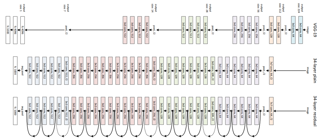
The above image is a representation of the Resnet architecture. In the following code block, we will implement the sample code that will fit on top of the output of the Resnet architecture.
# Input layer
input_layer = ResNet_MODEL.output

# Flatten
flatten = Flatten(data_format='channels_last',name='Flatten')(input_layer)

# Fully Connected layer-1
FC1 = Dense(units=30, activation='relu',
            kernel_initializer=keras.initializers.glorot_normal(seed=32),
            name='FC1')(flatten)

# Fully Connected layer-2
FC2 = Dense(units=30, activation='relu',
            kernel_initializer=keras.initializers.glorot_normal(seed=33),
            name='FC2')(FC1)

# Output layer
Out = Dense(units=num_classes, activation='softmax',
            kernel_initializer=keras.initializers.glorot_normal(seed=3),
            name='Output')(FC2)

model1 = Model(inputs=ResNet_MODEL.input,outputs=Out)
Model Summary and Plots
To analyze the model plot and summary for the ResNet model, use the following codes provided below. With the help of these models, you can analyze various factors accordingly. I chose not to include the summary and plot in this article because of their humungous size. Please feel free to check them out by yourselves with the codes provided for each of the following. The Jupyter Notebook attached below will contain the full code for these concepts as well.
model1.summary()The code for the model plot is as follows:
from tensorflow import keras
from keras.utils.vis_utils import plot_model

keras.utils.plot_model(model1, to_file='model1.png', show_layer_names=True)
2. InceptionV3
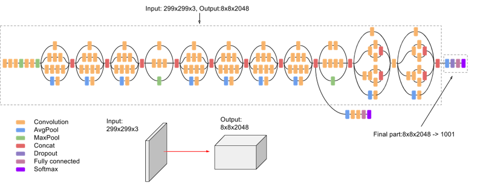
The above image is a representation of the InceptionV3 architecture. In the following code block, we will implement the sample code that will fit on top on the output of the InceptionV3 architecture.
# Input layer
input_layer = Inception_MODEL.output

# Flatten
flatten = Flatten(data_format='channels_last',name='Flatten')(input_layer)

# Fully Connected layer-1
FC1 = Dense(units=30, activation='relu',
            kernel_initializer=keras.initializers.glorot_normal(seed=32),
            name='FC1')(flatten)

# Fully Connected layer-2
FC2 = Dense(units=30, activation='relu',
            kernel_initializer=keras.initializers.glorot_normal(seed=33),
            name='FC2')(FC1)

# Output layer
Out = Dense(units=num_classes, activation='softmax',
            kernel_initializer=keras.initializers.glorot_normal(seed=3),
            name='Output')(FC2)


model2 = Model(inputs=Inception_MODEL.input,outputs=Out)
Model Summary And Plots
To analyze the model plot and summary for the InceptionV3 model, use the following codes provided below. With the help of these models, you can analyze various factors accordingly. I chose not to include the summary and plot in this article because of their humungous size. Please feel free to check them out by yourselves with the codes provided for each of the following. The Jupyter Notebook attached below will contain the full code for these concepts as well.
model2.summary()The code for the model plot is as follows:
from tensorflow import keras
from keras.utils.vis_utils import plot_model

keras.utils.plot_model(model2, to_file='model2.png', show_layer_names=True)
3. MobileNetV2
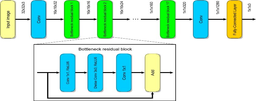
The above image is a representation of the MobileNetV2 architecture. In the following code block, we will implement the sample code that will fit on top on the output of the MobileNetV2 architecture.
# Input layer
input_layer = MobileNet_MODEL.output

# Flatten
flatten = Flatten(data_format='channels_last',name='Flatten')(input_layer)

# Fully Connected layer-1
FC1 = Dense(units=30, activation='relu',
            kernel_initializer=keras.initializers.glorot_normal(seed=32),
            name='FC1')(flatten)

# Fully Connected layer-2
FC2 = Dense(units=30, activation='relu',
            kernel_initializer=keras.initializers.glorot_normal(seed=33),
            name='FC2')(FC1)

# Output layer
Out = Dense(units=num_classes, activation='softmax',
            kernel_initializer=keras.initializers.glorot_normal(seed=3),
            name='Output')(FC2)

model3 = Model(inputs=MobileNet_MODEL.input,outputs=Out)
Model Summary and Plots
To analyze the model plot and summary for the MobileNetV2 model, use the following codes provided below. With the help of these models, you can analyze various factors accordingly. I chose not to include the summary and plot in this article because of their humungous size. Please feel free to check them out by yourselves with the codes provided for each of the following. The Jupyter Notebook attached below will contain the full code for these concepts as well.
model3.summary()The code for the model plot is as follows:
from tensorflow import keras
from keras.utils.vis_utils import plot_model

keras.utils.plot_model(model3, to_file='model3.png', show_layer_names=True)
Callbacks, Model Compilation, and Training
Now that we have completed building all the three models that we will be experimenting with our face recognition project with, let us proceed to define a few essential callbacks that might be useful for our task. In my code snippet, I have included the model checkpoints to save the best weights for each of the three models we plan to build, respectively. I have used the reduced learning rate and tensor board visualization callbacks but commented on them because I am training my models on only three models. Hence, I do not require their usage. Feel free to run more epochs and experiment accordingly. Refer to the code block below for defining the callbacks.
Defining the respective callbacks
from tensorflow.keras.callbacks import ModelCheckpoint
from tensorflow.keras.callbacks import ReduceLROnPlateau
from tensorflow.keras.callbacks import TensorBoard

checkpoint1 = ModelCheckpoint("face_rec1.h5", monitor='val_loss', save_best_only=True, mode='auto')

checkpoint2 = ModelCheckpoint("face_rec2.h5", monitor='val_loss', save_best_only=True, mode='auto')

checkpoint3 = ModelCheckpoint("face_rec3.h5", monitor='val_loss', save_best_only=True, mode='auto')

# reduce = ReduceLROnPlateau(monitor='val_loss', factor=0.2, patience=3, min_lr=0.00001, verbose = 1)

# logdir='logsface3'
# tensorboard_Visualization = TensorBoard(log_dir=logdir)
Compilation of the models
Now that we have defined all the necessary callbacks, we can proceed to the final two steps in the Jupyter Notebook, which is the compilation and fitting of the transfer learning models. The compilation stage is the configuration of the three models with the respective loss function, the most optimal optimizers, and the required metrics while performing the operation of fitting the models.
model1.compile(loss='categorical_crossentropy',
              optimizer=Adam(lr=0.00001),
              metrics=['accuracy'])

model2.compile(loss='categorical_crossentropy',
              optimizer=Adam(lr=0.00001),
              metrics=['accuracy'])

model3.compile(loss='categorical_crossentropy',
              optimizer=Adam(lr=0.00001),
              metrics=['accuracy'])
Fitting the Transfer Learning Models
We have completed all the necessary steps until this point to proceed with the training of each of our respective models. I implemented the training procedure for each of the respective models for a total of three epochs. Let us observe the outputs and draw a conclusion to the occurrences of these results.
1. ResNet 50
epochs = 3

model1.fit(train_generator,
           validation_data = validation_generator,
           epochs = epochs,
           callbacks = [checkpoint1])
#            callbacks = [checkpoint, reduce, tensorboard_Visualization])
Result
Train for 13 steps, validate for 4 steps
Epoch 1/3
13/13 [==============================] - 23s 2s/step - loss: 0.6726 - accuracy: 0.6498 - val_loss: 0.7583 - val_accuracy: 0.5000
Epoch 2/3
13/13 [==============================] - 16s 1s/step - loss: 0.3736 - accuracy: 0.8396 - val_loss: 0.7940 - val_accuracy: 0.5000
Epoch 3/3
13/13 [==============================] - 16s 1s/step - loss: 0.1984 - accuracy: 0.9332 - val_loss: 0.8568 - val_accuracy: 0.5000
2. InceptionV3
model2.fit(train_generator,
           validation_data = validation_generator,
           epochs = epochs,
           callbacks = [checkpoint2])
Result
Train for 13 steps, validate for 4 steps
Epoch 1/3
13/13 [==============================] - 21s 2s/step - loss: 0.6885 - accuracy: 0.5618 - val_loss: 0.8024 - val_accuracy: 0.4979
Epoch 2/3
13/13 [==============================] - 15s 1s/step - loss: 0.5837 - accuracy: 0.7122 - val_loss: 0.4575 - val_accuracy: 0.8090
Epoch 3/3
13/13 [==============================] - 15s 1s/step - loss: 0.4522 - accuracy: 0.8140 - val_loss: 0.3634 - val_accuracy: 0.8991
3. MobileNetV2
model3.fit(train_generator,
           validation_data = validation_generator,
           epochs = epochs,
           callbacks = [checkpoint3])
Result
Train for 13 steps, validate for 4 steps
Epoch 1/3
13/13 [==============================] - 17s 1s/step - loss: 0.7006 - accuracy: 0.5680 - val_loss: 0.7448 - val_accuracy: 0.5107
Epoch 2/3
13/13 [==============================] - 15s 1s/step - loss: 0.5536 - accuracy: 0.7347 - val_loss: 0.5324 - val_accuracy: 0.6803
Epoch 3/3
13/13 [==============================] - 14s 1s/step - loss: 0.4218 - accuracy: 0.8283 - val_loss: 0.4073 - val_accuracy: 0.7361
From the fitting and computation of these three transfer learning models, we can observe a few results. For the ResNet model, while the training accuracy and loss seem to keep improving, the validation accuracy remains unchanged. A few reasons for this occurrence could be due to the over-fitting of the large architecture on the smaller dataset. Another reason is due to the lack of depth in the fine-tuning architecture. It is recommended that you try out numerous parameters and a different fine-tuning architecture for obtaining better results. The results obtained for the inceptionV3 architecture and MobileNetV2 seem to be better in comparison to the ResNet50 architecture. Hence, we will utilize the saved checkpoint from the InceptionV3 model for the task of real-time prediction. The other improvements can be made by running more epochs, changing various parameters and other features, adding more layers, and just experimenting.
The final conclusion we can draw from this is that we have built three different types of performance models and understood their working functionality in further detail with a more practical approach.
Model Prediction
Once we have our model built and the best weights saved as a model in the .h5 format, we can utilize this resource. We can load the models saved with the checkpoint process and use them for the real-time identification of faces with the help of a webcam. The prediction stage is one of the more vital aspects of machine learning and deep learning because you have a clue on how the model you constructed will work in a real-time scenario. Let us import all the required libraries for the prediction of the real-time face recognition project.
Importing the libraries
from tensorflow.keras.models import load_model
from tensorflow.keras.preprocessing import image
from tensorflow.keras.preprocessing.image import ImageDataGenerator
from tensorflow.keras.preprocessing.image import img_to_array
import numpy as np
import cv2
import time
import os
Making the predictions in real-time
For the predictions in real-time, we will load our saved model for the best checkpoints and the haarcascade_frontalface_default.xml file for detecting the facial structures. We will then use the webcam for real-time face recognition. If the accuracy of the prediction is high, we will display the most suitable results. Most of the code structure is easy to understand, especially with the comment lines. You can feel free to experiment with the various modeling techniques or build a more convenient prediction setup if you deem it necessary.
model = load_model("face_rec2.h5")
face_classifier = cv2.CascadeClassifier('haarcascade_frontalface_default.xml')

Capture = cv2.VideoCapture(0)

while True:
    # Capture frame from the Video Recordings.
    ret, frame = Capture.read()

    # Detect the faces using the classifier.
    faces = face_classifier.detectMultiScale(frame,1.3,5)

    if faces is ():
        face = None

    # Create a for loop to draw a face around the detected face.
    for (x,y,w,h) in faces:
        # Syntax: cv2.rectangle(image, start_point, end_point, color, thickness)
        cv2.rectangle(frame, (x,y), (x+w,y+h), (0,255,255), 2)
        face = frame[y:y+h, x:x+w]

    # Check if the face embeddings is of type numpy array.
    if type(face) is np.ndarray:
        # Resize to (224, 224) and convert in to array to make it compatible with our model.
        face = cv2.resize(face,(224,224), interpolation=cv2.INTER_AREA)
        face = img_to_array(face)
        face = np.expand_dims(face, axis=0)

        # Make the Prediction.
        pred1 = model.predict(face)

        prediction = "Unknown"
        pred = np.argmax(pred1)

        # Check if the prediction matches a pre-exsisting model.
        if pred > 0.9:
            prediction = "Your_Name"

        elif pred < 0.9:
            prediction = "Other"

        else:
            prediction = "Unknown"

        label_position = (x, y)
        cv2.putText(frame, prediction, label_position, cv2.FONT_HERSHEY_SIMPLEX,2,(0,255,0),3)

    else:
        cv2.putText(frame, 'Access Denied', (20,60), cv2.FONT_HERSHEY_SIMPLEX,2,(0,255,0),3)

    cv2.imshow('Face Recognition', frame)

    if cv2.waitKey(1) & 0xFF == ord('q'):
            Capture.release()
            cv2.destroyAllWindows()

Capture.release()
cv2.destroyAllWindows()
You can go further with the exploration of the project and deploy the model either on a cloud environment, a raspberry pi, or any other similar embedded system, or your local desktop. Feel free to explore and build similar architectures to construct and develop a variety of tasks.
Conclusion

In this article, we started with the initial introduction of the numerous things that would be discussed and followed up with some general tips and suggestions. After the preliminary phase, we dived straight into the development of our project with the collection and pre-processing of our data for the construction of the different types of models. We then implemented the augmentation of the data to create more types of unique patterns. After this step, we proceeded to build our respective model architectures. Finally, we defined all the necessary callbacks for the required process before the compilation and the fitting of the model. We then programmed another code snippet for the real-time recognition of the respective faces to test the results that we receive.
I would highly recommend experimentation and implementation of other numerous methods of transfer learning or building your own custom network modeling systems to test how the results will pan out. Now that we have covered both the theoretical and practical aspects of understanding transfer learning network's work, you can go crazy with the computation of numerous other types of tasks. With the help of the resources provided in this article, you can easily implement all the three models utilized for performing the task of face recognition. In future articles, we will cover other topics related to deep learning and computer vision, such as image captioning, UNET, CANET, and so much more. Until then, then exploring and have fun!