Image Segmentation is one of the most intriguing and crucial aspects of any image recognition project because it is through image segmentation that we can determine the most essential elements and constituents in the particular picture. With image segmentation, the developers can separate the significant objects from other entities in the particular image. Once this extraction process is completed, we can either use the specified segment or the entire classified segmented image for numerous purposes and various applications. Isolating specific elements in an image can be used for determining abnormalities. Hence, image segmentation finds tremendous utility in biomedical tasks. However, the entire segmentation elements to learn about various parameters in the image can be used for other applications such as the road and vehicle segmentation data.
In our previous article, we understood the working and architecture of U-Net models. In this part, we will focus on another type of architectural building method to perform image segmentation tasks. The Chained Context Aggregation Network (CANet) is another fabulous approach for performing image segmentation tasks. It employs an asymmetric decoder to recover precise spatial details of prediction maps. This article is inspired by the research paper Attention-guided Chained Context Aggregation for Semantic Segmentation. This research paper covers most of the essential elements of this new technique of approach and how it can impact the performance of numerous complex tasks. If you are interested in learning almost every single element of this architecture, then it is recommended that you follow along with the entire article. However, if you want to focus on specific elements that you feel more interested in, then feel free to check out the table of contents.
Table of Contents:
- Introduction to CANet
- Brief Understanding of CAM and some loss functions
- Getting started with the architecture
1. Importing the libraries
2. Convolution block
3. Identity block
4. Verification of the shapes - Global Flow And Context Flow
- Feature Selection Module and Adapted Global Convolutional Network (AGCN)
- Finishing the build
- Conclusion
Introduction:
There are several methods, algorithms, and different types of architectures to solve numerous problems in deep learning. One such proposed architecture that solves the problem of image segmentation is the CANet model. This method utilizes the concept of making use of the fully convolutional network (FCN) similar to the U-Net architecture for capturing multi-scale contexts for obtaining precise localization and image segmentation masks. The proposed model introduces the concept of a series-parallel hybrid paradigm with the Chained Context Aggregation Module (CAM) to diversify feature propagation. The following new integration allows for the capturing of various spatial features and dimensions by a two-stage process, namely pre-fusion and re-fusion.
Apart from the previously discussed design characteristics, it also includes an encoder-decoder architecture where there is continuous downsampling of the input image in the encoder network. But in the decoder network, the data is upsampled back up to its original size. One major difference between the most common encoder-decoder architectural structures and the one used in the CANet model is that the CANet decoder is asymmetric while recovering precise spatial details of the prediction maps. They also use the concept of attention for obtaining the best possible results. The attention method is included alongside the CAM structure. Hence the term Chained Context Aggregation Network (CANet).
The key contributions of the CANet architecture include the chained context aggregation module for capturing multiple-scale features with the help of a series-parallel hybrid structure. The serial flow increasingly enlarges receptive fields of output neurons while parallel flows encode different region-based contexts, drastically improving the performance. The flow guidance enables the powerful aggregation of multi-scale contexts. The model is tested extensively on multiple challenging datasets and seems to provide the best results. Thus, it can be termed as one of the state-of-the-art performance methods.
Brief Understanding of CAM and some loss functions:
The Chained Context Aggregation Module (CAM) is one of the most critical aspects of the CANet architecture, as discussed previously. It consists of both the global flow and the context flow. Both of these structures are shallow encoder-decoder structures containing a down-sampling layer to gain different receptive fields, a projection layer to integrate sufficient context features, and an up-sampling layer to recover localization information.
When the global flow and the context flow are integrated as a series-parallel hybrid, they contribute to the high-quality encoding of multi-scale contexts. They have many advantages, including the large receptive features, the pixel features encoded at different shapes for image segmentation, high-quality encoding of multi-scale contexts, and simplifying the backpropagation of gradients. Let us now proceed to discuss some loss functions that are usually used for image segmentation tasks.
Learning about the dice loss and IoU loss:
Dice Loss is a popular loss function for image segmentation tasks, also referred to as the dice coefficient. It is essentially a measure of overlap between two samples.
Formulation =
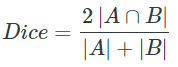
The range of the loss function is from 0 to 1 and it can be interpreted as follows:
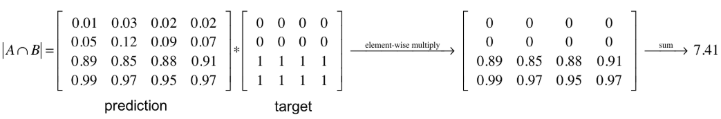
For the case of evaluating a Dice coefficient on predicted segmentation masks, we can approximate $|A∩B|$ as the element-wise multiplication between the prediction and target mask and then sum the resulting matrix. This loss function helps us to determine how much loss is encountered in each pixel and how accurate our model is performing per pixel. Then the overall sum can be taken to show the complete loss from a target model to the predicted model after segmentation is performed.
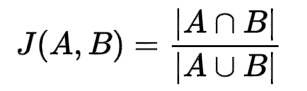
IoU score is another significant metric that is used for determining the quality of an image segmentation task. It is overall quite intuitive to interpret. A score of one is achieved through the predicted bounding box when it precisely matches the ground truth bounding box. A score of 0 means that the predicted bounding box and the true bounding box of the ground truth do not overlap at all. The computation for the IoU score is as follows:
Getting started with the architecture:
The implementation of the CANet architecture from scratch is quite complex. We have several coding blocks that we need to focus on with high precision to achieve the best results and ensure we are obtaining the best results. We will create custom classes to perform most of the operations as described in the original research paper. This method of constructing architectures with the TensorFlow and Keras deep learning frameworks is also referred to as model sub-classing. Before we start constructing each segment of the architecture from scratch, check out the entire model that we will construct and all the essential entities that it encompasses.
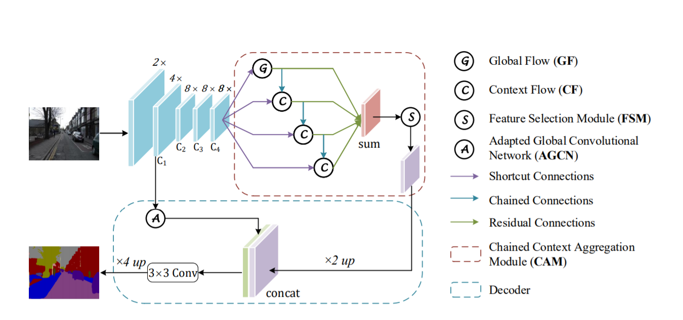
The above diagram is a representation of the things to come ahead. The upper and lower parts of this architectural design can be considered as two parts, namely the encoder and the decoder. In the encoder structure, we have the convolutional blocks and the identity blocks alongside other elements like Global Flow, Context Flow, and the feature selection block, where the initial input image which is passed through the model is continuously downsampled as we are considering only the image sizes with widths and heights less than the original image.
Once we pass it through the decoder block, all these elements are upsampled once again to get the desired output, which is in most cases the same size as the input. Let us get started with the construction of the CANet architecture. Please follow along carefully as some parts might be slightly confusing and easy to get stuck on. We will proceed by importing all the required libraries for the particular task and move on to the convolution and identity blocks.
import tensorflow as tf
# tf.compat.v1.enable_eager_execution()
from tensorflow import keras
from tensorflow.keras.layers import *
from tensorflow.keras.preprocessing import image
from tensorflow.keras.models import Model, load_model
from tensorflow.keras.layers import UpSampling2D
from tensorflow.keras.layers import MaxPooling2D, GlobalAveragePooling2D
from tensorflow.keras.layers import concatenate
from tensorflow.keras.layers import Multiply
from tensorflow.keras.callbacks import EarlyStopping, ModelCheckpoint
from tensorflow.keras import backend as K
from tensorflow.keras.layers import Input, Add, Dense, Activation, ZeroPadding2D, BatchNormalization, Flatten, Conv2D, AveragePooling2D, MaxPooling2D, GlobalMaxPooling2D
from tensorflow.keras.models import Model, load_model
from tensorflow.keras.utils import plot_model
from tensorflow.keras.initializers import glorot_uniform
K.set_image_data_format('channels_last')
K.set_learning_phase(1)
Convolution Blocks:
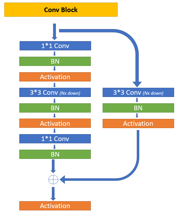
The first step in the CANet model is to take the input image and pass it through the convolutional block and apply a max-pooling layer with a stride of two. However, this code is a single convolutional layer, and it is not repeated again through the architecture. Hence, we will keep the initial convolutional layer, which processes the input image separately in the final architecture. In this section, we will construct the iterative convolutional block.
The next step of the architecture is to create the channel maps in the encoder build with the convolution blocks C1, C2, C3, C4. For performing this operation we will utilize the convolution block class with the respective subclass modeling methods to obtain the best results possible. It is crucial to note that the images that are passed through the convolution architectures have decreasing shapes. They are as follows.
- C1 width and heights are 4x times less than the original image.
- C2 width and heights are 8x times less than the original image.
- C3 width and heights are 8x times less than the original image.
- C4 width and heights are 8x times less than the original image.
The below code block is a representation of how this procedure can be successfully accomplished.
class convolutional_block(tf.keras.layers.Layer):
    def __init__(self, kernel=3,  filters=[4,4,8], stride=1, name="conv block"):
        super().__init__(convolutional_block)
        self.F1, self.F2, self.F3 = filters
        self.kernel = kernel
        self.stride = stride

        self.conv_1 = Conv2D(self.F1,(1,1),strides=(self.stride,self.stride),padding='same')
        self.conv_2 = Conv2D(self.F2,(self.kernel,self.kernel),strides=(1,1),padding='same')
        self.conv_3 = Conv2D(self.F3,(1,1),strides=(1,1),padding='same')
        self.conv_4 = Conv2D(self.F3,(self.kernel,self.kernel),strides=(self.stride,self.stride),padding='same')

        self.bn1 = BatchNormalization(axis=3)
        self.bn2 = BatchNormalization(axis=3)
        self.bn3 = BatchNormalization(axis=3)
        self.bn4 = BatchNormalization(axis=3)

        self.activation = Activation("relu")

        self.add = Add()

    def call(self, X):
        # write the architecutre that was mentioned above

        X_input = X

        # First Convolutional Block

        conv1 = self.conv_1(X)
        bn1 = self.bn1(conv1)
        act1 = self.activation(bn1)

        # Second Convolutional Block

        conv2 = self.conv_2(act1)
        bn2 = self.bn2(conv2)
        act2 = self.activation(bn2)

        # Third Convolutional Block

        conv3 = self.conv_3(act2)
        bn3 = self.bn3(conv3)

        # Adjusting the input

        X_input = self.conv_4(X_input)
        X_input = self.bn4(X_input)
        X_input = self.activation(X_input)

        # Re-add the input

        X = self.add([bn3, X_input])
        X = self.activation(X)

        return X
Identity Block:
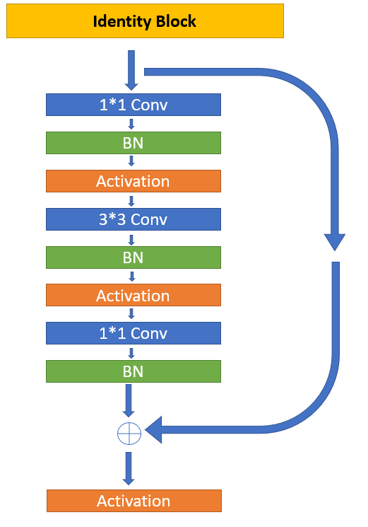
The identity block is used in the architecture when we know that the input and output dimensions must be preserved. It is a method often used to preserve the entities while also being an approach to avoid the bottleneck of the features of the model. The convolutional blocks C1, C2, C3, and C4 are formed by applying a convolutional block followed by $k$ number of identity block. This means the $C(k)$ feature map will consist of a single convolutional block followed by $k$ number of identity blocks. The code below is a representation of how you can perform this operation quite easily.
class identity_block(tf.keras.layers.Layer):
    def __init__(self, kernel=3,  filters=[4,4,8], name="identity block"):
        super().__init__(identity_block)
        self.F1, self.F2, self.F3 = filters
        self.kernel = kernel

        self.conv_1 = Conv2D(self.F1, (1,1), (1,1), padding="same")
        self.conv_2 = Conv2D(self.F2, (self.kernel,self.kernel), (1,1), padding="same")
        self.conv_3 = Conv2D(self.F3, (1,1), (1,1), padding="same")

        self.bn1 = BatchNormalization(axis=3)
        self.bn2 = BatchNormalization(axis=3)
        self.bn3 = BatchNormalization(axis=3)

        self.activation = Activation("relu")

        self.add = Add()


    def call(self, X):
        # write the architecutre that was mentioned above

        X_input = X

        conv1 = self.conv_1(X)
        bn1 = self.bn1(conv1)
        act1 = self.activation(bn1)

        conv2 = self.conv_2(act1)
        bn2 = self.bn2(conv2)
        act2 = self.activation(bn2)

        conv3 = self.conv_3(act2)
        bn3 = self.bn3(conv3)

        X = self.add([bn3, X_input])
        X = self.activation(X)


        return X
Verification of the shapes:
In this section, we will quickly construct the starting of the initial architecture and test the progress of our build with the help of an image shape. This step is done once to check if the progress of your development models is accurate and matches up accordingly. From the next sections, we will not repeat this step, but you are free to try them out by yourself.
X_input = Input(shape=(256,256,3))

# Stage 1
X = Conv2D(64, (3, 3), name='conv1', padding="same", kernel_initializer=glorot_uniform(seed=0))(X_input)
X = BatchNormalization(axis=3, name='bn_conv1')(X)
X = Activation('relu')(X)
X = MaxPooling2D((2, 2), strides=(2, 2))(X)
print(X.shape)

# First Convolutional Block

c1 = convolutional_block(kernel=3,  filters=[4,4,8], stride=2)(X)
print("C1 Shape = ", c1.shape)

I11 = identity_block()(c1)
print("I11 Shape = ", I11.shape)

# Second Convolutional Block

c2 = convolutional_block(kernel=3,  filters=[8,8,16], stride=2)(I11)
print("C2 Shape = ", c2.shape)

I21 = identity_block(kernel=3,  filters=[8,8,16])(c2)
print("I21 Shape = ", I21.shape)

I22 = identity_block(kernel=3,  filters=[8,8,16])(I21)
print("I22 Shape = ", I22.shape)

# Third Convolutional Block

c3 = convolutional_block(kernel=3,  filters=[16,16,32], stride=1)(I22)
print("C3 Shape = ", c3.shape)

I31 = identity_block(kernel=3,  filters=[16,16,32])(c3)
print("I31 Shape = ", I31.shape)

I32 = identity_block(kernel=3,  filters=[16,16,32])(I31)
print("I32 Shape = ", I32.shape)

I33 = identity_block(kernel=3,  filters=[16,16,32])(I32)
print("I33 Shape = ", I33.shape)

# Fourth Convolutional Block

c4 = convolutional_block(kernel=3,  filters=[32,32,64], stride=1)(I33)
print("C3 Shape = ", c4.shape)

I41 = identity_block(kernel=3,  filters=[32,32,64])(c4)
print("I41 Shape = ", I41.shape)

I42 = identity_block(kernel=3,  filters=[32,32,64])(I41)
print("I42 Shape = ", I42.shape)

I43 = identity_block(kernel=3,  filters=[32,32,64])(I42)
print("I43 Shape = ", I43.shape)

I44 = identity_block(kernel=3,  filters=[32,32,64])(I42)
print("I44 Shape = ", I44.shape)
Output:
(None, 128, 128, 64)
C1 Shape =  (None, 64, 64, 8)
I11 Shape =  (None, 64, 64, 8)
C2 Shape =  (None, 32, 32, 16)
I21 Shape =  (None, 32, 32, 16)
I22 Shape =  (None, 32, 32, 16)
C3 Shape =  (None, 32, 32, 32)
I31 Shape =  (None, 32, 32, 32)
I32 Shape =  (None, 32, 32, 32)
I33 Shape =  (None, 32, 32, 32)
C3 Shape =  (None, 32, 32, 64)
I41 Shape =  (None, 32, 32, 64)
I42 Shape =  (None, 32, 32, 64)
I43 Shape =  (None, 32, 32, 64)
I44 Shape =  (None, 32, 32, 64)
Now that we have a brief idea that we are on the right track because all our image shapes seem to match up perfectly, we can proceed towards the next sections of the article to implement the further steps of the CANet model architecture.
Global Flow And Context Flow:
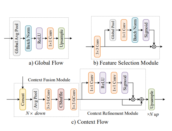
As shown in the above image representation, we will utilize the global average pooling architecture for starting the construction of the global flow. This function computes the global average for the entire spatial dimensional data. We then pass this information through the next blocks, which are the Batch Normalization layer, the ReLU activation function, and the 1x1 Convolutional layer. The final output shape we obtain is in the format of (None, 1, 1, number of filters). We can then pass these values through an upsample layer with bilinear pooling as an interpolation technique or a Conv2D transpose layer (as we did in the previous article).
class global_flow(tf.keras.layers.Layer):
    def __init__(self, input_dim, output_dim, channels, name="global_flow"):
        super().__init__(global_flow)

        self.input_dim = input_dim
        self.output_dim = output_dim
        self.channels = channels

        self.conv1 = Conv2D(64,kernel_size=(1,1),strides=(1,1),padding='same')
        self.global_avg_pool = GlobalAveragePooling2D()
        self.bn = BatchNormalization(axis=3)
        self.activation = Activation("relu")
        self.upsample = UpSampling2D(size=(self.input_dim,self.output_dim),interpolation='bilinear')

    def call(self, X):
        # implement the global flow operatiom

        global_avg = self.global_avg_pool(X)

        global_avg= tf.expand_dims(global_avg, 1)
        global_avg = tf.expand_dims(global_avg, 1)

        bn1 = self.bn(global_avg)
        act1 = self.activation(bn1)

        conv1 = self.conv1(act1)

        X = self.upsample(conv1)

        return X
For the context flow, we have the context fusion module where we take the output from the C4 convolution block and the output from the global flow to concatenate them together as one unit. We then proceed to apply the average pooling and the convolutional layers. We can skip the channel shuffling as it is not really required. Then, we have the context refinement module where the following operation is performed before upsampling (or running it through a Conv2D transpose layer) -
$$Y=(X⊗σ((1∗1)conv(relu((1∗1)conv(X)))))⊕X$$
class context_flow(tf.keras.layers.Layer):
    def __init__(self, name="context_flow"):
        super().__init__(context_flow)

        self.conv_1 = Conv2D(64, kernel_size=(3,3), strides=(1,1), padding="same")
        self.conv_2 = Conv2D(64, kernel_size=(3,3), strides=(1,1), padding="same")
        self.conv_3 = Conv2D(64, kernel_size=(1,1), strides=(1,1), padding="same")
        self.conv_4 = Conv2D(64, kernel_size=(1,1), strides=(1,1), padding="same")

        self.concatenate = Concatenate()

        self.avg_pool = AveragePooling2D(pool_size=(2,2))

        self.activation_relu = Activation("relu")
        self.activation_sigmoid = Activation("sigmoid")

        self.add = Add()
        self.multiply = Multiply()

        self.upsample = UpSampling2D(size=(2,2),interpolation='bilinear')


    def call(self, X):

        # here X will a list of two elements
        INP, FLOW = X[0], X[1]

        # implement the context flow as mentioned in the above cell

        # Context Fusion Module

        concat = self.concatenate([INP, FLOW])
        avg_pooling = self.avg_pool(concat)
        conv1 = self.conv_1(avg_pooling)
        conv2 = self.conv_2(conv1)

        # Context Refinement Module

        conv3 = self.conv_3(conv2)
        act1 = self.activation_relu(conv3)
        conv4 = self.conv_4(act1)
        act2 = self.activation_sigmoid(conv4)

        # Combining and upsampling

        multi = self.multiply([conv2, act2])
        add = self.add([conv2, multi])
        X = self.upsample(add)

        return X
You can perform the shape verification after this step as well for an optional assessment to ensure that you are currently on the right track. Once you ensure that there is no shape mismatch, you can proceed to the further sections to implement the next few blocks.
Feature Selection Module and Adapted Global Convolutional Network (AGCN):
The next couple of code blocks that we will construct are comparatively smaller in size and easier to understand. This method is similar to the working of an attention layer where we have the input pass through a convolutional layer. And the output of the convolutional layer obtained is divided into two segments. The first one is passed through some layers containing a sigmoid function, and the other one is multiplied by the output of the sigmoid layer.
class fsm(tf.keras.layers.Layer):
    def __init__(self, name="feature_selection"):
        super().__init__(fsm)

        self.conv_1 = Conv2D(32, (3,3), (1,1), padding="same")
        self.global_avg_pool = GlobalAveragePooling2D()
        self.conv_2 = Conv2D(32 ,kernel_size=(1,1),padding='same')
        self.bn = BatchNormalization()
        self.act_sigmoid = Activation('sigmoid')
        self.multiply = Multiply()
        self.upsample = UpSampling2D(size=(2,2),interpolation='bilinear')

    def call(self, X):

        X = self.conv_1(X)
        global_avg = self.global_avg_pool(X)
        global_avg= tf.expand_dims(global_avg, 1)
        global_avg = tf.expand_dims(global_avg, 1)
        conv1= self.conv_2(global_avg)
        bn1= self.bn(conv1)
        Y = self.act_sigmoid(bn1)
        output = self.multiply([X, Y])
        FSM_Conv_T = self.upsample(output)

        return FSM_Conv_T
The next structure that we will look at is the Adapted Global Convolutional Network (AGCN).
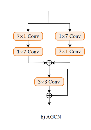
The AGCN block will receive the input from the output of the convolutional block of C1. In all the above layers, we will be using the padding = "same" and set the strides as (1,1). Hence the final input and output matrices obtained are of the same size. Let us explore the code block to view the implementation.
class agcn(tf.keras.layers.Layer):
    def __init__(self, name="global_conv_net"):
        super().__init__(agcn)
        self.conv_1  = Conv2D(32,kernel_size=(1,7),padding='same')
        self.conv_2  = Conv2D(32,kernel_size=(7,1),padding='same')
        self.conv_3  = Conv2D(32,kernel_size=(1,7),padding='same')
        self.conv_4  = Conv2D(32,kernel_size=(7,1),padding='same')
        self.conv_5  = Conv2D(32,kernel_size=(3,3),padding='same')
        self.add = Add()

    def call(self, X):
        # please implement the above mentioned architecture
        conv1 = self.conv_1(X)
        conv2= self.conv_2(conv1)

        # side path
        conv3 = self.conv_4(X)
        conv4 = self.conv_3(conv3)

        add1 = self.add([conv2,conv4])

        conv5 = self.conv_5(add1)

        X = self.add([conv5,add1])

        return X
Now that we have completed the construction of the entire architecture, the final step of the model building is to ensure that we have accomplished the desired results. The best way to find the working procedure is to pass an image size through the architecture as the input size and verify the following results. If these shapes match the ones you have manually calculated through downsampling and upsampling, then the final upsampled output that results is the original image size. This image size will be the exact same as the input except with the total number of features/classes replacing the RGB or grayscale channel.
X_input = Input(shape=(512,512,3))

# Stage 1
X = Conv2D(64, (3, 3), name='conv1', padding="same", kernel_initializer=glorot_uniform(seed=0))(X_input)
X = BatchNormalization(axis=3, name='bn_conv1')(X)
X = Activation('relu')(X)
X = MaxPooling2D((2, 2), strides=(2, 2))(X)
print(X.shape)

# First Convolutional Block

c1 = convolutional_block(kernel=3,  filters=[4,4,8], stride=2)(X)
print("C1 Shape = ", c1.shape)

I11 = identity_block()(c1)
print("I11 Shape = ", I11.shape)

# Second Convolutional Block

c2 = convolutional_block(kernel=3,  filters=[8,8,16], stride=2)(I11)
print("C2 Shape = ", c2.shape)

I21 = identity_block(kernel=3,  filters=[8,8,16])(c2)
print("I21 Shape = ", I21.shape)

I22 = identity_block(kernel=3,  filters=[8,8,16])(I21)
print("I22 Shape = ", I22.shape)

# Third Convolutional Block

c3 = convolutional_block(kernel=3,  filters=[16,16,32], stride=1)(I22)
print("C3 Shape = ", c3.shape)

I31 = identity_block(kernel=3,  filters=[16,16,32])(c3)
print("I31 Shape = ", I31.shape)

I32 = identity_block(kernel=3,  filters=[16,16,32])(I31)
print("I32 Shape = ", I32.shape)

I33 = identity_block(kernel=3,  filters=[16,16,32])(I32)
print("I33 Shape = ", I33.shape)

# Fourth Convolutional Block

c4 = convolutional_block(kernel=3,  filters=[32,32,64], stride=1)(I33)
print("C3 Shape = ", c4.shape)

I41 = identity_block(kernel=3,  filters=[32,32,64])(c4)
print("I41 Shape = ", I41.shape)

I42 = identity_block(kernel=3,  filters=[32,32,64])(I41)
print("I42 Shape = ", I42.shape)

I43 = identity_block(kernel=3,  filters=[32,32,64])(I42)
print("I43 Shape = ", I43.shape)

I44 = identity_block(kernel=3,  filters=[32,32,64])(I42)
print("I44 Shape = ", I44.shape)

# Global Flow

input_dim = I44.shape[1]
output_dim = I44.shape[2]
channels = I44.shape[-1]

GF1 = global_flow(input_dim, output_dim, channels)(I44)
print("Global Flow Shape = ", GF1.shape)

# Context Flow 1

Y = [I44, GF1]
CF1 = context_flow()(Y)
print("CF1 shape = ", CF1.shape)

# Context Flow 2

Z = [I44, CF1]
CF2 = context_flow()(Y)
print("CF2 shape = ", CF2.shape)

# Context Flow 3

W = [I44, CF1]
CF3 = context_flow()(W)
print("CF3 shape = ", CF3.shape)

# FSM Module

out = Add()([GF1, CF1, CF2, CF3])
print("Sum of Everything = ", out.shape)
fsm1 = fsm()(out)
print("Shape of FSM = ", fsm1.shape)

# AGCN Module

agcn1 = agcn()(c1)
print("Shape of AGCN = ", agcn1.shape)

# Concatinating FSM and AGCN

concat = Concatenate()([fsm1, agcn1])
print("Concatinated Shape = ", concat.shape)

# Final Convolutional Block

final_conv = Conv2D(filters=21, kernel_size=(1,1), strides=(1,1), padding="same")(concat)
print("Final Convolution Shape = ", final_conv.shape)

# Upsample

up_samp = UpSampling2D((4,4), interpolation="bilinear")(final_conv)
print("Final Shape = ", up_samp.shape)

# Activation

output = Activation("softmax")(up_samp)
print("Final Shape = ", output.shape)
Output:
(None, 256, 256, 64)
C1 Shape =  (None, 128, 128, 8)
I11 Shape =  (None, 128, 128, 8)
C2 Shape =  (None, 64, 64, 16)
I21 Shape =  (None, 64, 64, 16)
I22 Shape =  (None, 64, 64, 16)
C3 Shape =  (None, 64, 64, 32)
I31 Shape =  (None, 64, 64, 32)
I32 Shape =  (None, 64, 64, 32)
I33 Shape =  (None, 64, 64, 32)
C3 Shape =  (None, 64, 64, 64)
I41 Shape =  (None, 64, 64, 64)
I42 Shape =  (None, 64, 64, 64)
I43 Shape =  (None, 64, 64, 64)
I44 Shape =  (None, 64, 64, 64)
Global Flow Shape =  (None, 64, 64, 64)
CF1 shape =  (None, 64, 64, 64)
CF2 shape =  (None, 64, 64, 64)
CF3 shape =  (None, 64, 64, 64)
Sum of Everything =  (None, 64, 64, 64)
Shape of FSM =  (None, 128, 128, 32)
Shape of AGCN =  (None, 128, 128, 32)
Concatinated Shape =  (None, 128, 128, 64)
Final Convolution Shape =  (None, 128, 128, 21)
Final Shape =  (None, 512, 512, 21)
Final Shape =  (None, 512, 512, 21)
The CANet model plot is also attached to this article. Feel free to view it if you have any confusion.
Finishing the build:
Now that we have successfully built the complete architecture of the CANet model from scratch with the help of our own custom methods by defining each of the elements from scratch, we are free to save, load, and utilize this saved model on any kind of dataset. You will need to figure out the appropriate methods to load the data accordingly. An example of this can be referred to from the previous article on U-Net. We solved an example project with the help of the Sequence class in the Keras deep learning framework. We can also use data generators for loading the data. Below is an example code on how to utilize the constructed CANet architecture. You will load the model, call the required scores for computation, define the optimizers, compile, and finally, train (fit) the model on the particular task.
model = Model(inputs = X_input, outputs = output)
import segmentation_models as sm
from segmentation_models.metrics import iou_score
optim = tf.keras.optimizers.Adam(0.0001)
focal_loss = sm.losses.cce_dice_loss
model.compile(optim, focal_loss, metrics=[iou_score])
history = model.fit(train_dataloader,
validation_data=test_dataloader,
epochs=5,
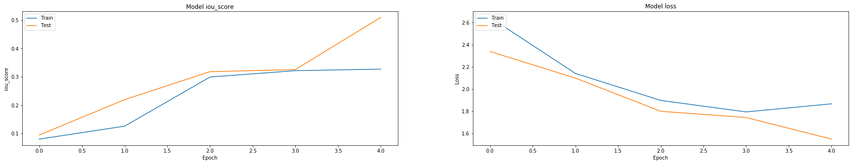
callbacks=callbacks1)After the computation of my project on the dataset, I was able to achieve the following IoU scores. The graphical representation for both the IoU of the model as well as the loss for the model is displayed below. To re-iterate, this graph is from an example project that I solved on the road segmentation dataset. You can choose to experiment on your own as well on different types of datasets.
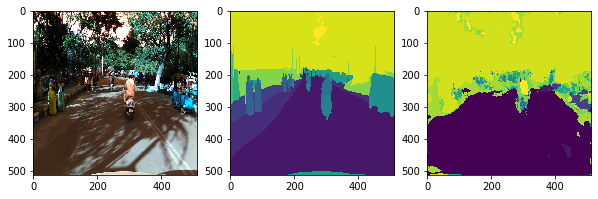
The image displayed below is one of the final image segmentation outputs for the appropriate input image. As we can notice, it does a pretty decent job in the segmentation process.
If you are interested in building amazing and unique projects with CANet for image segmentation, there are tons of options available for you to implement. As an example, you can check out a similar kind of project from the following GitHub link. Have fun exploring and constructing unique projects on your own with this architectural build!
Conclusion:
Computer Vision and deep learning are at its highest peak right now. Their superior applications and capability to achieve almost any task that was once deemed impossible for machines to achieve is commendable with the vast progress made in these respective fields. One such task that holds equivalently high significance in comparison to other tasks is the problem of image segmentation. While the U-Net architecture designed and introduced in the year 2015 was able to achieve high-quality results and win a multitude of prizes, we have advanced further since then. Many recreations, modifications, and innovations to this model have been made. Once such method we discussed and understood in this article is the architecture of the Chained Context Aggregation Network (CANet) model.
In this article, we understood the concept of CANet and the numerous elements in the design process. We always looked briefly into some of the significant topics in the CANet model and briefly understood the aspects of the loss functions, namely the dice loss and the IoU score. After these sections, we proceeded to construct the overall complex architecture of the CANet architecture. We explored all the various entities that constitute this model. These include the input layer with the convolutional network, the convolutional blocks, the identity blocks, the global flow and context flow, the feature selection block, and the Adapted Global Convolutional Network (AGCN). Finally, we verified all the appropriate shapes accordingly for the entire architecture. We then looked at a sample project output that shows the outstanding results the CANet model can produce on the image segmentation tasks.
With the help of this architecture and the U-Net model discussed in the previous article, you can accomplish a lot of tasks. It is highly recommended that you try out numerous projects with both this architecture to see their performance. In the upcoming articles, we will cover topics of image captioning and DCGANs. Until then, keep coding and have fun!


