Interpreting Computer Vision Models

Computer Vision as a field dates back to the late 1960s, when it originated with the ambitious goal of mimicking the human visual system. However, after a long AI winter, the field recently came into spotlight in 2012 when AlexNet won the first ImageNet Challenge. AlexNet used deep CNNs on GPUs to classify millions of images in ImageNet along with thousands of labels with a top 5 error rate of 15.3%.

Some of you may be wondering: what are CNNs?

Let me explain it to you briefly.

The connectivity pattern between neurons in a Convolutional Neural Networks or CNN is inspired by the organization of the animal visual cortex. Individual neurons in the cortex respond to stimuli only in a restricted region of the visual field called the receptive field. Similarly, CNNs have kernels(an n x n matrix with shared weights) that slides along the input image to capture spatial information that a Multi-layer perceptron won't.

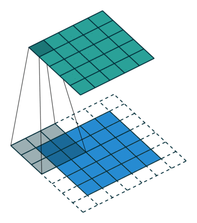
For a high resolution image, it was computationally unfeasible to have a network of fully connected nodes. Also, full connectivity of neurons is wasteful for images that inherently contains spatially local input patterns. We can infer from the patterns finer details, and save on cost.

The rise of CNNs and the case for interpretability

CNNs, while reducing the network size, also add locality of reference, which is very important for image data. As a result, CNNs are widely used for computer vision tasks.

• In self driving cars, for example, they are used for everything from detecting and classifying objects on the road to segmenting road from the sidewalk.
• In healthcare, they are used on X-rays, MRIs and CT scans to detect ailments.
• They are also used in manufacturing and production lines to detect defected products.

These are only a few use cases among many, but they rightly convey how interwoven these systems are with our daily lives these days. But, while they are common, their interpretation can be difficult with out in domain knowledge of deep learning and AI. Therefore, it has become extremely important to be able to explain the predictions of these "black boxes". In this blog, we will explore techniques to interpret the predictions made by these networks.

I will broadly divide the interpretation techniques into two categories:

Occlusion or perturbation based techniques

These methods manipulate parts of the image to generate explanations. How exactly does that work? I'll explain it using two libraries.

1. LIME Image Explainer:

Local Interpretable Model Agnostic Explanation(or LIME) is a library that supports local explanations for almost all modalities of data. These explanations are model-agnostic (independent of the model used), and try to explain only individual predictions and not the whole model (local). The way LIME works for images can be broken down in the following steps:

• Get random perturbations of the image: In LIME, variations of the images are generated by segmenting the image into "superpixels" and turning them off or on. These superpixels are interconnected, and can be turned off by replacing each pixel with gray. For each image, we have a set of perturbed images.
• Predicting classes for perturbed images: For each perturbed image, a class is predicted using the original model that we are trying to interpret.
• Computing the importance of the perturbations: A distance metric such as cosine similarity is used to evaluate how different each perturbation is from the original image. The original image is also a perturbation with all the superpixels on.
• Training an explainable surrogate model: A surrogate model is a linear model like logistic regression that is intrinsically interpretable. This model takes in the input and output of the original model and tries to approximate the original model. The initial weights are the weights we calculated in the last step. After the model is fit, the weights or the coefficients associated with each superpixel in the image tell us how important that superpixel was for the predicted class.

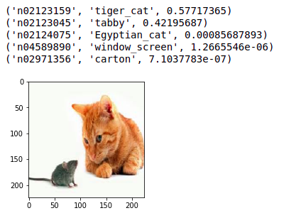
We'll now use a pretrained Inception-V3 model to make a prediction on a cat and mouse image.

from keras.applications import inception_v3 as inc_net
from keras.preprocessing import image
from keras.applications.imagenet_utils import decode_predictions
from skimage.io import imread
import matplotlib.pyplot as plt
import lime
from lime import lime_image

def load_img(path):
    img = image.load_img(path, target_size=(224, 224))
    img = image.img_to_array(img)
    img = np.expand_dims(img, axis=0)
    return img

def predict_class(img):
    img = inc_net.preprocess_input(img)
    img = np.vstack([img])
    return inet_model.predict(img)

inet_model = inc_net.InceptionV3()

img = load_img('cat-and-mouse.jpg')
preds = predict_class(img)
plt.figure(figsize=(3,3))
plt.imshow(img[0] / 2 + 0.5)
for x in decode_predictions(preds)[0]:
    print(x)

Next, we'll interpret these predictions using LIME.

# instantiate lime image explainer and get the explaination 
explainer = lime_image.LimeImageExplainer()
explanation = explainer.explain_instance(img[0], inet_model.predict, top_labels=5, hide_color=0, num_samples=1000)

# plot interpretation
temp, mask = explanation.get_image_and_mask(282, positive_only=False, num_features=100, hide_rest=False)
plt.figure(figsize=(3,3))
plt.imshow(skimage.segmentation.mark_boundaries(temp / 2 + 0.5, mask))

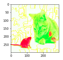
The green super-pixels contribute positively towards the predicted label i.e. tiger cat. While the red super-pixels contribute negatively.

Even though some red super-pixels lie on the cat. The model does a pretty good job at learning the underlying concept in the image, and the colorations reflect that.

Lime's implementation for images is quite similar to its implementation for tabular data. But instead of  perturbing individual pixels, we change super-pixels. Because of the locality reference that we talked about earlier, many more than one pixel contribute to a class.

2. SHAP Partition Explainer:

Another popular library for interpretations is SHAP. It uses concepts from game theory to generate explanations. Consider a game played by a group of individuals where they cooperate. Each player contributes something to the game, some players may contribute more than others and some players may contribute negatively. There will be a final distribution of the summation of each player's contribution that will determine the outcome of the game.

We want to know how important each player is to the overall cooperation and what payoff they can expect. To make it more specific to the task at hand, how important is each super-pixel's contribution to the overall predicted class of the image.

Shapley value provides one possible answer to it.

Let's try to use SHAP to interpret the same cat and mouse image. Here we'll use a Resnet50 instead of an Inception model.

from tensorflow.keras.applications.resnet50 import ResNet50, preprocess_input
import shap
import json 

# load pretrained model
model = ResNet50(weights='imagenet')
def predict(x):
    tmp = x.copy()
    preprocess_input(tmp)
    return model(tmp)

# get imagenet class names
url = "https://s3.amazonaws.com/deep-learning-models/image-models/imagenet_class_index.json"
with open(shap.datasets.cache(url)) as file:
    class_names = [v[1] for v in json.load(file).values()]

# define a masker that is used to mask out partitions of the input image.
masker = shap.maskers.Image("inpaint_telea", img.shape[1:])

# create an explainer with model and image masker
explainer = shap.Explainer(f, masker, output_names=class_names,algorithm='partition')

# here we explain the same image and use 1000 evaluations of Resnet50 to get the shap values 
shap_values = explainer(img, max_evals=1000, batch_size=50, outputs=shap.Explanation.argsort.flip[:4])

shap.image_plot(shap_values)

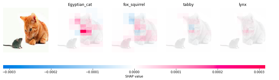
The first predicted class is Egyptian cat followed by fox squirrel, tabby and lynx. The superpixels of the face of the cat contribute positively towards the prediction. The model places a great weight on the nose or the whiskers area.

An advantage of using the Partition explainer in SHAP is it does not make an underlying assumption that the features(or superpixels) here exist independently from other features. This is a very big (and false) assumption made by a lot of interpretation models out there.

We'll now look at the next class of interpretation techniques.

Gradient Based Techniques

These methods compute the gradient of the prediction with respect to the input image. Simply put, they find out whether a change in the pixel would change the prediction. If you were to change the color value of a pixel, the predicted class probability would either go up(positive gradient) or go down(negative gradient). The magnitude of the gradient tells us the importance of our perturbation.

We'll look at a few techniques that use gradients for interpretation:

1. Grad-CAM

Gradient Weighted Class Activation map or Grad-CAM uses the gradients of a class flowing into the final convolutional layer to produce a heatmap that highlights the important regions in the image used for predicting the class. This heatmap is then upscaled and superimposed over the input image to get the visualization. The steps followed to get the heatmap are as follows:

1. We forward-propogate the image through the network to get the predictions, and also the activations of the last convolutional layer, before the fully connected layer.
2. Then we compute the gradient of the top predicted class with respect to the activations of the last convolutional layer.
3. We then weigh each feature map pixel by the gradient of the class. This gives us globally pooled gradients.
4. We calculate an average of the feature maps which is weighted per pixel by the gradient. This is done by multiplying the each channel in the feature map obtained in the last map with the output of the last layer. This tells us how important the channel is with regard to  the output class. Then we sum all the channels to get the heatmap activation for that class.
5. We then normalize the pixels between 0 and 1, so that it's easy to visualize.

import tensorflow as tf
import keras
import matplotlib.cm as cm
from IPython.display import Image

def make_gradcam_heatmap(img_array, model, LAST_CONV_LAYER_NAME, pred_index=None):
    # Step 1
    grad_model = tf.keras.models.Model(
        [model.inputs], [model.get_layer(LAST_CONV_LAYER_NAME).output, model.output]
    )
    
    with tf.GradientTape() as tape:
        last_conv_layer_output, preds = grad_model(img_array)
        if pred_index is None:
            pred_index = tf.argmax(preds[0])
        class_channel = preds[:, pred_index]

    # Step 2
    grads = tape.gradient(class_channel, last_conv_layer_output)

    # Step 3
    pooled_grads = tf.reduce_mean(grads, axis=(0, 1, 2))

    # Step 4
    last_conv_layer_output = last_conv_layer_output[0]
    heatmap = last_conv_layer_output @ pooled_grads[..., tf.newaxis]
    heatmap = tf.squeeze(heatmap)

    # Step 5
    heatmap = tf.maximum(heatmap, 0) / tf.math.reduce_max(heatmap)
    return heatmap.numpy()

We use the same ResNet50 model that we have used in the above example. We also have a helper function that superimposes the heatmap on the original image and displays it.

def save_and_display_gradcam(img_path, heatmap, alpha=0.4):
    # Load the original image
    img = keras.preprocessing.image.load_img(img_path)
    img = keras.preprocessing.image.img_to_array(img)

    # Rescale heatmap to a range 0-255
    heatmap = np.uint8(255 * heatmap)

    # Use jet colormap to colorize heatmap
    jet = cm.get_cmap("jet")

    # Use RGB values of the colormap
    jet_colors = jet(np.arange(256))[:, :3]
    jet_heatmap = jet_colors[heatmap]

    # Create an image with RGB colorized heatmap
    jet_heatmap = keras.preprocessing.image.array_to_img(jet_heatmap)
    jet_heatmap = jet_heatmap.resize((img.shape[1], img.shape[0]))
    jet_heatmap = keras.preprocessing.image.img_to_array(jet_heatmap)

    # Superimpose the heatmap on original image
    superimposed_img = jet_heatmap * alpha + img
    superimposed_img = keras.preprocessing.image.array_to_img(superimposed_img)
    # Display the image
    plt.figure(figsize=(8,4))
    plt.axis("off")
    plt.imshow(superimposed_img)

Tired of the cat and mouse image? We'll use a new image this time.

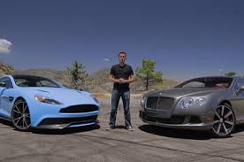
Let's look at the top classes for this image.

# Prepare image
img_array = preprocess_input(load_img('cars.jpg',224))
# Print the top 2 predicted classes
preds = model.predict(img_array)
print("Predicted:", decode_predictions(preds, top=2)[0])

The model classifies the cars as sports car and the person standing between them as a racer. Let's visualize the activations of the last convolutional layer.

heatmap = make_gradcam_heatmap(img_array, model, 'conv5_block3_out', pred_index=class_names.index("sports_car"))
save_and_display_gradcam('cars.jpg', heatmap)

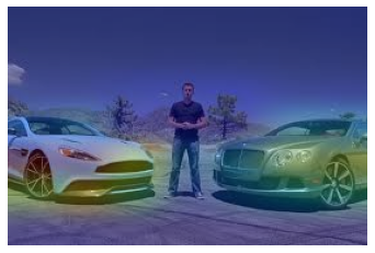
It seems like the neurons of the layer conv5_block3_out are activated by the front portion of the car. We can be assured that the model learns the right features for this class.

Now, let's visualize this for the "racer" class.

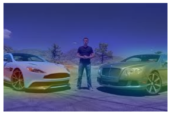
This time instead of giving importance to the pixels representing the man the car still uses the car pixels for classifying this image as "racer". This is not in-line with what we expected and maybe the model uses global context in the image to predict classes. For instance- would a person not standing besides a sports car be called a racer?

That's for you to find out ;)

2. Guided Grad-CAM

Since Grad CAM uses the last convolutional layer to generate the heatmap, the localization is very coarse. Since the last layer has a much coarser resolution compared to the input image, the heatmap is upscaled before it can be superimposed on the image.

We use guided backpropogation to get a high resolution localization. Instead of computing the gradients of loss with regard to the activations of the last convolutional layer we compute it with regard to the pixels of the input image. However, doing this can produce a noisy image, and therefore we use ReLu in backpropogation (in other words, we clip all values less than 0).

@tf.custom_gradient
def guided_relu(x):
    # guided version of relu which allows only postive gradients in backpropogation
    def grad(dy):
        return tf.cast(dy > 0, "float32") * tf.cast(x > 0, "float32") * dy

    return tf.nn.relu(x), grad

class GuidedBackprop:
    def __init__(self, model):
        self.model = model
        self.gb_model = self.build_guided_model()

    def build_guided_model(self):
        # build a guided version of the model by replacing ReLU with guided ReLU in all layers
        gb_model = tf.keras.Model(
            self.model.inputs, self.model.output
        )
        layers = [
            layer for layer in gb_model.layers[1:] if hasattr(layer, "activation")
        ]
        for layer in layers:
            if layer.activation == tf.keras.activations.relu:
                layer.activation = guided_relu
        return gb_model

    def guided_backprop(self, image: np.ndarray, class_index: int):
        # convert to one hot representation to match our softmax activation in the model definition
        expected_output = tf.one_hot([class_index] * image.shape[0], NUM_CLASSES)
        # define the loss
        with tf.GradientTape() as tape:
            inputs = tf.cast(image, tf.float32)
            tape.watch(inputs)
            outputs = self.gb_model(inputs)
            loss = tf.keras.losses.categorical_crossentropy(
                expected_output, outputs
            )
        # get the gradient of the loss with respect to the input image
        grads = tape.gradient(loss, inputs)[0]
        return grads

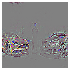
Let's take a look at the saliency map for the sports car example that we saw above. We'll use the same ResNet50 model.

gb = GuidedBackprop(model)
NUM_CLASSES = 1000
saliency_map = gb.guided_backprop(img_array, class_index=class_names.index("sports_car")).numpy()

# Normalize with mean 0 and std 1
saliency_map -= saliency_map.mean()
saliency_map /= saliency_map.std() + tf.keras.backend.epsilon()
# Change mean to 0.5 and std to 0.25
saliency_map *= 0.25
saliency_map += 0.5
# Clip values between 0 and 1
saliency_map = np.clip(saliency_map, 0, 1)
# Change values between 0 and 255
saliency_map *= (2 ** 8) - 1
saliency_map = saliency_map.astype(np.uint8)

plt.axis('off')
plt.imshow(saliency_map)

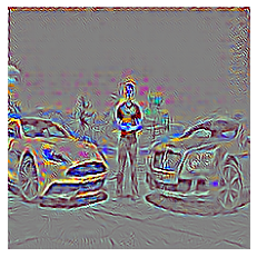
Even though the saliency map we created through guided backpropagation is higher resolution, it is not class discriminative, i.e. the localization cannot differentiate between classes. That's where we use Grad-CAM. The Grad-CAM heatmap is upsampled with bilinear interpolation, then both maps are multiplied element-wise.

gb = GuidedBackprop(model)

# Guided grad_cam is just guided backpropogation with feature importance coming from grad-cam
saliency_map = gb.guided_backprop(img_array, class_index=class_names.index("sports_car")).numpy()
gradcam = cv2.resize(heatmap, (224, 224))
gradcam =
np.clip(gradcam, 0, np.max(gradcam)) / np.max(gradcam)
guided_gradcam = saliency_map * np.repeat(gradcam[..., np.newaxis], 3, axis=2)

# Normalize
guided_gradcam -= guided_gradcam.mean()
guided_gradcam /= guided_gradcam.std() + tf.keras.backend.epsilon()
guided_gradcam *= 0.25
guided_gradcam += 0.5
guided_gradcam = np.clip(guided_gradcam, 0, 1)
guided_gradcam *= (2 ** 8) - 1
guided_gradcam = guided_gradcam.astype(np.uint8)

plt.axis('off')
plt.imshow(guided_gradcam)

Grad-CAM works like a lens that focuses on specific parts of the pixel-wise attribution map obtained through guided backpropagation. Here, for the class "sports car", mostly the pixels related to the cars are highlighted.

gb = GuidedBackprop(model)

# Guided grad_cam is just guided backpropogation with feature importance coming from grad-cam
saliency_map = gb.guided_backprop(img_array, class_index=class_names.index("racer")).numpy()
gradcam = cv2.resize(heatmap, (224, 224))
gradcam = np.clip(gradcam, 0, np.max(gradcam)) / np.max(gradcam)
guided_gradcam = saliency_map * np.repeat(gradcam[..., np.newaxis], 3, axis=2)

# Normalize
guided_gradcam -= guided_gradcam.mean()
guided_gradcam /= guided_gradcam.std() + tf.keras.backend.epsilon()
guided_gradcam *= 0.25
guided_gradcam += 0.5
guided_gradcam = np.clip(guided_gradcam, 0, 1)
guided_gradcam *= (2 ** 8) - 1
guided_gradcam = guided_gradcam.astype(np.uint8)

plt.axis('off')
plt.imshow(guided_gradcam)

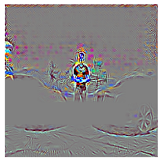
As you can see, guided Grad CAM does a better job at localizing the pixels for the class "racer" than just Grad CAM.

3. Expected Gradients

Next in line are expected gradients. They combine three different concepts: one of which you have already heard about in SHAP values. Along with SHAP values, they use Integrated gradients.  Integrated gradients values are a little different from SHAP values, and require a single reference value to integrate from. To make them approximate SHAP values, in expected gradients we reformulate the integral as an expectation, and combine that expectation with reference values sampled from the background dataset. This leads to a single combined expectation of gradients that converges toward attribution values which sum up to give the difference between the expected model output and the current output.

The last concept it uses is Local Smoothing. It adds normally distributed noise with the standard deviation (specified as an argument) during the expectation calculation. This helps create smoother feature attributions that better capture correlated regions of the image.

We'll use VGG16 this time, and, since we have visualized gradients from the input image and the last convolutional layer, we'll visualize gradients from an intermediate layer (layer 7).

from keras.applications.vgg16 import VGG16
from keras.applications.vgg16 import preprocess_input, decode_predictions
import tensorflow.compat.v1.keras.backend as K
import tensorflow as tf
tf.compat.v1.disable_eager_execution()

# load pre-trained model and choose two images to explain
model = VGG16(weights='imagenet', include_top=True)
X,y = shap.datasets.imagenet50()
to_explain = load_img('cars.jpg',224)

# load the ImageNet class names
url = "https://s3.amazonaws.com/deep-learning-models/image-models/imagenet_class_index.json"
fname = shap.datasets.cache(url)
with open(fname) as f:
    class_names = json.load(f)
    
# explain how the input to the 7th layer of the model explains the top two classes
def map2layer(x, layer):
    feed_dict = dict(zip([model.layers[0].input], [preprocess_input(x.copy())]))
    return K.get_session().run(model.layers[layer].input, feed_dict)

e = shap.GradientExplainer((model.layers[7].input, model.layers[-1].output), map2layer(preprocess_input(X.copy()), 7) ,local_smoothing=100)
shap_values,indexes = e.shap_values(map2layer(to_explain, 7), ranked_outputs=3, nsamples=100)

# get the names for the classes
index_names = np.vectorize(lambda x: class_names[str(x)][1])(indexes)

# plot the explanations
shap.image_plot(shap_values, to_explain, index_names)

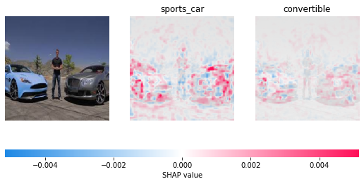
The first label predicted by the model is sports car. The 7th layer of the model pays attention to the pixels highlighted in red.

Conclusion

We looked at various techniques to visualize CNNs. Something to note here is, when the explanations provided by the model do not match our expectations it could be because of two reasons. Either the model did not learn correctly or the model learned more complex relationships than can be  perceived by humans.

Try this out on a Gradient Notebook by creating a TensorFlow Runtime Notebook with the following as your 'Workspace URL' in the 'Advanced Options' of Notebook creation: https://github.com/gradient-ai/interpretable-ml-keras

References

• https://shap.readthedocs.io/en/latest/generated/shap.explainers.Partition.html
• https://shap.readthedocs.io/en/stable/example_notebooks/image_examples/image_classification/Explain ResNet50 using the Partition explainer.html
• https://towardsdatascience.com/interpretable-machine-learning-for-image-classification-with-lime-ea947e82ca13
• https://towardsdatascience.com/interpreting-cnn-models-a11b1f720097
• https://shap-lrjball.readthedocs.io/en/latest/example_notebooks/gradient_explainer/Explain an Intermediate Layer of VGG16 on ImageNet.html