Bring this project to life
Introduction
XGBoost, which stands for eXtreme Gradient Boosting, is a Machine Learning algorithm that has made a significant impact in the field of Data Science (DS), Machine Learning (ML) and predictive modeling. XGBoost, a tree based ML algorithm, was developed in the year 2014. This powerful and versatile algorithm, authored by Tianqi Chen, has gained immense popularity because of its high-efficiency and achievement of state-of-the-art results on many ML challenges.
In this article, we will provide an overview of the XGBoost algorithm, its key features, and highlight the significant impact it has had on various applications in data-driven fields. Additionally, we have incorporated a case study in our article, demonstrating XGBoost through our Paperspace platform. This case study utilizes a dataset akin to that used in the original research paper.
Overview
Improving the accuracy of Machine Learning algorithms involves more than merely fitting the models and generating predictions. Many successful ML models at both the industry and competition levels have leveraged Ensemble Techniques and Feature Engineering to enhance their performance.
XGBoost can be called as an optimized distributed boosting library, designed to be highly efficient, flexible and portable. It is implemented under the Gradient Boosting framework. Considering the ML competitions hosted on platforms like Kaggle, Hackerrank, or CodeWars, it's noteworthy that among the top challenge-winning solutions approximately 60% employed XGBoost as a crucial component. Within this group of solutions, ~27% exclusively relied on XGBoost for model training, While the majority of others adopted a strategy of combining XGBoost with neural networks within ensemble models.
In order to understand XGBoost it is important to understand a few important ML components, such as supervised learning, decision trees, ensemble learning and gradient boosting.
Supervised Machine Learning can be defined as using algorithms to trains a model to find patterns in a dataset with labels and features. This trained model is then used to predict the labels on a new dataset’s features or known as the test data which is unseen to the model.
Decision trees construct a predictive model by creating a tree-like structure of true/false feature-based on if-then-else questions. This algorithm aims to determine the minimal number of inquiries required to estimate the likelihood of arriving at an accurate decision. These trees find applications in classification, where they forecast category labels, as well as in regression, where they predict continuous numerical values.
A Gradient Boosting Decision Trees (GBDT) is a decision tree based on ensemble learning algorithm, for classification and regression. Ensemble learning algorithms combine multiple Machine Learning algorithms to obtain a better model. The term Gradient Boosting comes from the word "Boosting" which involves combining several weak learners which collectively builds strong models.
Key features and advantages of XGBoost
XGBoost is a versatile framework which is compatible with multiple programming languages, including R, Python, Julia, C++, or any language of an individual's preference. This algorithm exhibits high portability, allowing seamless integration with diverse systems like the Paperspace platform, Azure, or Colab. Notably, when utilizing the Paperspace platform, users benefit from the convenience of running the algorithm on a wide selection of available GPUs.
These are just a few highlights of this popular framework. The reason that makes the algorithm so popular are not just these highlights, but also the speed of processing and the outputs it produces (or performance) known as 2P's. These 2P's constitute the key features of XGBoost. The improved performance of XGBoost is attributed to its foundation built upon Gradient Boosting (GB). To put it succinctly, XGBoost represents a significant enhancement over GB that surpasses alternative ensemble learning methods like Random Forest (RF), primarily due to its strong emphasis on what we can call the "2P's."
Now what makes this algorithm so fast?
The answer lies behind the concept of parallelization, where the decision trees that create the ensemble are computed using parallel processes. If the algorithm runs on a single processor, then all the cores of the CPU are taken into account. And if it runs on a distributed mode, it ensures to use the maximum available computation power of the system.
Another reason behind the speed of the algorithm is cache optimization. Caches are a ubiquitous feature in computer systems, employed for various purposes, such as web browsers storing frequently accessed web pages. The fundamental objective of caching is to expedite data retrieval, resulting in enhanced system efficiency and responsiveness. Cache serves as a high-speed data access mechanism and serves as an intermediary layer between the CPU and the main memory. In the case of XGBoost, it efficiently retains intermediate computations and statistical information, allowing for rapid predictions to be generated with remarkable speed and efficiency.
However, this is just the processing part, as a data scientist one is also concerned about the performance part. In this algorithm, there is a concept of regularization and auto-pruning which prevents the model from overfitting. This criteria is not present in GB. A regularization parameter is passed while calling the model which makes sure overfitting is handled. Hence, the variance of the model is controlled. Also, auto-pruning is a feature which does not lead the model to grow beyond a certain depth. This automatic process of trimming or removing specific branches or subtrees from the gradient boosting decision tree during its construction prevents overfitting, which occurs when a decision tree becomes overly complex and fits the training data too closely, leading to poor generalization on unseen data.
These exceptional features make the model robust, furthermore XGBoost takes care of the missing values. In the research paper , the author stated that the algorithm seamlessly accommodates sparse feature formats. XGBoost uses a sparsity-aware algorithm to find optimal splits in decision trees, where at each split the feature set is selected randomly with replacement. When a missing value is encountered, XGBoost can make an informed decision about whether to go left or right in the tree structure based on the available data. This is particularly useful for categorical features with missing values.
Internally, XGBoost learns the best direction to go when a value is missing. This process takes place during the training phase.
This is the reason that makes the algorithm most popular ML algorithms among AI practitioners, Data Scientist, and ML engineers.
Prerequisites and Notes for XGBoost
XGBoost can be installed easily using pip. On Paperspace, this package is already installed, though you may want to upgrade the package.
# Pip 21.3+ is required
pip install -U xgboost
if we run into permission errors. One can run the command with --user flag or use virtualenv
It is worth noting that XGBoost requires DLLs from Visual C++ Redistributable in order to function, so make sure to install it. Exception: If Visual Studio installed, then all necessary libraries are installed, which eliminates the need to install the Visual C++ Redistributable separately. This however is not necessary on Paperspace.
We may also use the Conda packaging manager to install XGBoost:
conda install -c conda-forge py-xgboostThe py-xgboost-gpu is currently not available on Windows. Windows users may need to use pip to install XGBoost with GPU support.
XGBoost Simplified: A Quick Overview

In this section of the tutorial, we will look at a few of the key features of XGBoost in detail. For information about the mathematical equations underlying the model structures, check out this section from an older Paperspace Blog tutorial.
Boosting
As we learned, XGBoost is a refined iteration of the Boosting algorithm, serving as its foundational core. Boosting is an ensemble modeling method aimed at constructing a robust classifier by combining several weak classifiers. A series of weak learners are combined to build a model. Initially, a model is constructed using the training data. Subsequently, a second model is created with the objective of rectifying any errors made by the first model. This process is iterated, and models are incorporated until either the entire training dataset is predicted accurately or the maximum allowable number of models are reached.
Gradient Boosting
Gradient Boosting is a Machine Learning technique that focuses on improving the predictive performance of models by training multiple weak learners, typically decision trees built sequentially. The key idea behind gradient boosting is to correct the errors made by the previous models in an iterative manner.
XGBoost
In this algorithm, decision trees are created sequentially and weights play a major role in XGBoost. In this approach, each independent variable is initially assigned weights and input into a decision tree for prediction. Variables predicted incorrectly by the tree receive increased weights and are subsequently used in a second decision tree. These individual classifiers then combine to create a robust and more accurate model through ensemble learning.
This iterative approach of boosting which adapts and improves the model over time, effectively reducing prediction errors and creating a strong ensemble model. It is widely used for both regression and classification tasks and is known for its high predictive accuracy. Popular implementations of gradient boosting include XGBoost, LightGBM, and CatBoost.
XGBoost Parameters
XGBoost has a wide range of parameters that can be tuned to customize the behavior and performance of the model. Let's take a look at some of these before identifying which are most important to potentially adjust during training.
- General Parameters:
- booster: Type of boosting model (gbtree, gblinear), the default option is gbtree
- silent: Verbosity level, the valid values are 0 (silent), 1 (warning), 2 (info), 3 (debug). Verbosity is known to print messages
- nthread: Number of parallel CPU threads to use for processing
- Tree Booster Parameters:
- eta (or learning_rate): Default value is 0.3, This value is the step size shrinkage to prevent overfitting
- max_depth: Maximum depth of the tree
- min_child_weight: Specifies the minimum total weight of all observations necessary in a child node. This parameter controls overfitting however a higher value can result in under fitting
- subsample: Fraction of observations used for building tree building. This occurs once in every iteration
- colsample_bytree: Fraction of features or columns used for tree building
- lambda (or reg_lambda): L2 regularization
- alpha (or reg_alpha): L1 regularization
- Learning Task Parameters:
- objective: Here the default value reg:squarederror, Objective defines the loss function which the model aim to reduces (e.g., reg:squarederror for regression, binary:logistic for binary classification)
- eval_metric: Evaluation metric to monitor during training (e.g., rmse for regression, logloss for binary classification)
- Control Parameters:
- num_round (or n_estimators): Number of boosting rounds (trees)
- early_stopping_rounds: If the validation metric doesn't improve for a specified number of rounds, training stops
- Cross-Validation Parameters:
- num_folds (or nfolds): Number of cross-validation folds
- stratified: Perform stratified sampling for cross-validation. This is used when there is a imbalance in classes in the target variable
These are just a selection of the many parameters available in XGBoost. The choice of parameters depends on the specific problem and the dataset. Careful tuning these parameters can significantly impact the model's performance.
- Additional Parameters:
- scale_pos_weight: The default value is 1. This parameter creates a balance of positive and negative weights.
- seed: Random seed for reproducibility.
- gamma: Minimum loss reduction required to make a further partition on a leaf node.
How to best adjust XGBoost parameters for optimal training
Adjusting the parameters for optimal training involves a combination of understanding the problem statement, the dataset and hyperparameter tuning.
- The first step before diving into hyperparameter tuning is to understand the dataset and the problem statement. This should include initial data preparation, feature engineering, Exploratory Data Analysis (EDA), and settling with the evaluation metric depending upon the problem (classification or regression)
- Splitting the data into train, test and validation which can be used to train the model and test its performance on the other two sets. During this process one should also keep in mind the data leakage issue. Creating the model using the train set, evaluating the model in the test set and validating the model using the validation set after finding the best hyperparameter. This ensures an unbiased estimate of its performance
- Creating a base model first with the important or the default parameters. This provides a good starting point for the model and later fine tune the parameters for better performance of the model
- Next, perform the hyperparameter tuning using techniques like Grid Search, Random Search, or Bayesian optimization (e.g., using libraries like GridSearchCV or RandomizedSearchCV in scikit-learn, or Optuna)
Among the many parameters XGBoost has, a few of them are most important and need to be considered when deploying a model for training. Here is a list of parameters for optimal training.A. Learning rate (eta) B. Maximum depth (max_depth)C. Number of trees (n_estimators)D. Minimum child weight (min_child_weight)E. Gamma (min_split_loss)F. Subsampling and column subsamplingG. Early stoppingH. Cross-validation
- Implement early stopping
- Experiment with regularization technique such as L1 and L2
- Feature selection and understanding of each feature plays a major role. Identifying the main features plays a crucial role. XGBoost has a built-in feature importance score that can help with this. Or we can use tools like SHAP or LIME. These libraries can help find the important features which are contributing positively towards the model. And, helps in explaining the black box model
- After achieving a satisfactory level of performance with the model, it's crucial to deploy it for real-world predictions. However, ongoing monitoring is essential because the data environment can evolve over time. This necessitates periodic retraining of the model to account for changing data distributions and new requirements. Even when the model has initially fine-tuned the hyperparameters and struck a balance, it's common to revisit and potentially revamp the hyperparameters. This iterative process remains a fundamental aspect of Data Science, reflecting its adaptability to dynamic data landscapes
Please keep in mind that the optimal set of hyperparameters may vary from one problem to another. It's essential to strike a balance between bias and variance, and this is often called a bias variance trade-off.
Why choose paperspace GPU
Using GPUs (Graphics Processing Units) for XGBoost can provide several advantages, making it a compelling choice for certain scenarios.
- GPUs provide parallel computing and can perform many calculations simultaneously compared to CPUs. XGBoost, like other gradient boosting algorithms, involves a lot of parallelizable calculations. Using GPUs can significantly speed up the training process
- GPUs can be an effective solution while working with larger datasets which include a high number of features. It is also feasible to train XGBoost with large number of defined parameter on datasets that might be impractical to process using only CPUs
- XGBoost models are known to be computationally intensive and can be called complex models. Ensemble model includes a large number of deep trees, and GPU acceleration can help reduce training times significantly
- GPU-accelerated XGBoost can make it possible to generate predictions quickly, ensuring timely responses to user queries or data processing requirements
Paperspace is a cloud computing platform that offers GPU instances, making it a popular choice for various tasks, including Machine Learning and Data Science.
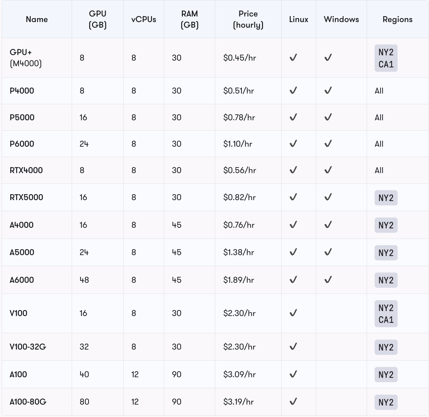
A wide range of GPUs provided by Paperspace such as NVIDIA GPUs like the V100, P100, and A100. This can be particularly valuable for tasks such as XGBoost that require extensive computational power. Each machine includes a 50 GB SSD by default and can be expanded up to 2 TB. Here is a list of dedicated GPUs including the price are provided below:-
Furthermore, Paperspace also provides Multi-GPU that are variants of dedicated GPU machines with up to 8 GPUs. These specs and pricing can be simply doubled, quadrupled, and so on, from the base machine type. The user-friendly interface simplifies the process of setting up the environment and getting started quickly.
Types
- P4000x2, P4000x4
- P5000x2, P5000x4
- P6000x2, P6000x4
- RTX4000x2, RTX4000x4
- RTX5000x2, RTX5000x4
- V100-32Gx2, V100-32Gx4
- A4000x2, A4000x4
- A5000x2, A5000x4
- A6000x2, A6000x4
- A100x2, A100x4, A100x8
- A100-80Gx2, A100-80Gx4, A100-80Gx8
The V100-32Gx2, V100-32Gx4, and A100-80Gx8 machine types offer NVLink support to facilitate the Multi-GPU setups. Note that the x8 setups are limited to Core Machines, and inaccessible for use with Notebooks.
To add more one can easily start a Jupyter notebook on GPU instances, making it a popular choice for data scientists and Machine Learning practitioners who prefer using Jupyter for development and experimentation.
The platform is also affordable because of a range of pricing options, including both pay-as-you-go and subscription plans. This flexibility allows users to choose a plan that best suits their budget and project requirements.
Also one should note that GPU need depends on the specific dataset and problem. Not all tasks will experience a significant speedup, and XGBoost can be easily trained on a CPU enabled system. It's advisable to perform benchmarking to assess the actual performance and evaluate whether the associated costs are justified by the speed and efficiency improvements. However, Paperspace can be a valuable resource for individuals, teams, and organizations looking to leverage GPU acceleration for their A.I., Data Science and Machine Learning tasks in a cloud-based environment.
Implementation of Extreme Gradient Boosting using Python in Paperspace Console
Here, we'll guide you through a step-by-step demonstration of how to use XGBoost to tackle a real-world problem. While the original research paper utilized four datasets, we've employed a comparable dataset in this tutorial to showcase XGBoost in action.
| Dataset | Task |
|---|---|
| Allstate | Insurance claim classification |
| Higgs Boson | Event classification |
| Yahoo LTRC | Learning to Rank |
| Criteo | Click through rate prediction |
Code Demo and explanation
Bring this project to life
Let us now walk through how to download the dataset, create the model, and utilize it for predicting outcomes on test data.
Please click the provided link to access the Paperspace console, and from there, choose the "XGBoost_final.ipynb" file to open the notebook.
The below code loads the dataset from the web. Here, we will use a classification problem predicting the click-through Rate. The purpose of click-through rate (CTR) prediction is to predict how likely a person will click on an advertisement or item.
url="https://raw.githubusercontent.com/ataislucky/Data-Science/main/dataset/ad_ctr.csv"
ad_data = pd.read_csv(url)
Explaining the Features of the dataset in brief
The code displays the columns or the features present in the dataset.
ad_data.columnsVariables present in the data set are:
- Clicked on Ad : 1 if the user clicked on the ad, else 0;
- Age : the age of the user
- Daily Time Spent on Site: the daily time spent by the user on the website
- Daily Internet Usage: Internet usage of the user
- Area Income: average income of the user
- City: city
- Ad Topic Line: title of the ad
- Timestamp:time when the user visited the website
- Gender:gender of the user
- Country:country of the user
Data Preparation and Analysis
The below piece of code snippet displays the shape of the dataset, basic info, data types, and value counts of the target column.
# provides the dtypes of the columns
ad_data.dtypes
# prints the shape of the dataframe
ad_data.shape
# displays the columns present in the data
ad_data.columns
# describes the dataframe
ad_data.describe()
Categorical columns need to be converted into numerical columns before feeding into the model.
gender_mapping = {'Male': 0, 'Female': 1}
ad_data['Gender'] = ad_data['Gender'].map(gender_mapping)
ad_data['Gender'].value_counts(normalize=True)
# Use Label Encoding to convert 'country' to numerical feature
ad_data['Country'] = ad_data['Country'].astype('category').cat.codes
ad_data['Country'].value_counts()
Dropping few unnecessary columns before model training
ad_data.drop(['Ad Topic Line','City','Timestamp'],axis=1, inplace=True)Randomly split training set into train and test subsets
X_train,X_test,y_train,y_test=train_test_split(X,y,test_size=0.2,random_state=45)
X_train.shape,X_test.shape,y_train.shape,y_test.shape
Model Training Build XGBoost Model and Make Predictions
It is imperative to divide our dataset into two distinct sets: the training set, which is used to train our model, and the testing set, which serves to evaluate how effectively our model fits the dataset.
Once the split is done we move to train the base model, here we are using the default parameter for training the model to show its effectiveness.
# Step 4: Create and train the first basic XGBoost model
model = XGBClassifier()
model.fit(X_train, y_train)
Once trained we will use the model to predict the test data set and evaluate its performance on the test data set.
# Step 5: Make predictions
y_pred = model.predict(X_test)
The below code evaluates the model performance.
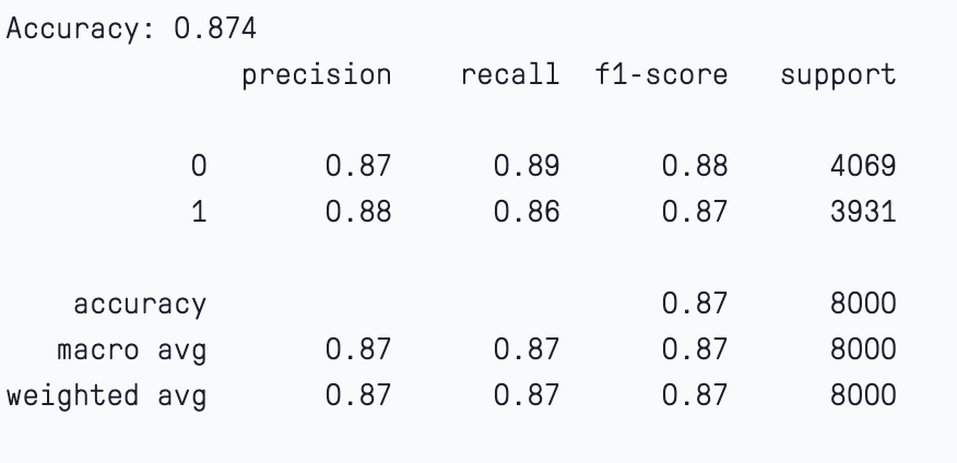
# Step 6: Evaluate the model's performance
accuracy = accuracy_score(y_test, y_pred)
print(f"Accuracy: {accuracy:.2f}")
print(classification_report(y_test, y_pred))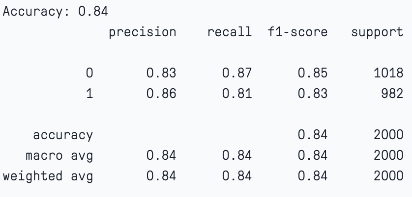
Here, we notice that by providing the default parameters the model has worked quite well. Please note that accuracy alone may not be a reliable parameter for judging the performance of a machine learning classification model.
Hyperparameter tuning and finding the best parameter
Hyperparameter tuning in XGBoost is a crucial step to optimize the performance of your model. Here are the key steps and considerations for XGBoost hyperparameter tuning:
To find the best parameter we will use GridSearchCV and Randomized search CV. The below code is used to train the model and find the best parameters.
PARAMETERS = {"subsample":[0.5, 0.75, 1],
"colsample_bytree":[0.5, 0.75, 1],
"max_depth":[2, 6, 12],
"min_child_weight":[1,5,15],
"learning_rate":[0.3, 0.1, 0.03],
"n_estimators":[100]}
model = XGBClassifier(n_estimators=100, n_jobs=-1, eval_metric='error')
"""Initialise Grid Search Model to inherit from the XGBoost Model,
set the of cross validations to 3 per combination and use accuracy
to score the models."""
model_gs = GridSearchCV(model,param_grid=PARAMETERS,cv=3,scoring="accuracy")model_gs.fit(X_train,y_train)
print(model_gs.best_params_)
Once we get the best parameter from GrisSearchCV, we use those parameters to further train and fit the model.
#Initialise model using best parameters
model = XGBClassifier(objective="binary:logistic",subsample=1,
colsample_bytree=0.5,
min_child_weight=1,
max_depth=12,
learning_rate=0.1,
n_estimators=100)
#Fit the model but stop early if there has been no reduction in error after 10 epochs.
model.fit(X_train, y_train, early_stopping_rounds=5, eval_set=[(X_test, y_test)])
Use the model to predict the target variable on the unseen data.
train_predictions = model.predict(X_train)
model_eval(y_train, train_predictions)
Next, we will again pass the parameters and this time we will also add the regularization parameter.
params = {'max_depth': [3, 6, 10, 15],
              'learning_rate': [0.01, 0.1, 0.2, 0.3, 0.4],
              'subsample': np.arange(0.5, 1.0, 0.1),
              'colsample_bytree': np.arange(0.5, 1.0, 0.1),
              'colsample_bylevel': np.arange(0.5, 1.0, 0.1),
              'n_estimators': [100, 250, 500, 750],
              'reg_alpha' : [0.1,0.001,.00001],
              'reg_lambda': [0.1,0.001,.00001]

              }
Instantiate the model, with 100 estimators.
xgbclf = XGBClassifier(n_estimators=100, n_jobs=-1)Here, we use RandomizedCV to find the best parameter.
clf = RandomizedSearchCV(estimator=xgbclf,
                             param_distributions=params,
                             scoring='accuracy',
                             n_iter=25,
                             n_jobs=4,
                             verbose=1)
Fit the model, find the best parameter and use it to predict the target variable.
clf.fit(X_train,y_train)
print("Best hyperparameter combination: ", clf.best_params_)
Repeat the process to train and test the model.
#Initialise model using best parameters from randomized cv
model_new_hyper = XGBClassifier(
subsample=0.89,
reg_alpha=0.1, # L1 regularization (Lasso)
reg_lambda=0.1, # L2 regularization (Ridge)
colsample_bytree=0.6,
colsample_bylevel=.8,
min_child_weight=1,
max_depth=3,
learning_rate=0.2,
n_estimators=500)
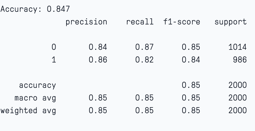
#Fit the model but stop early if there has been no reduction in error after 10 epochs.
model_new_hyper.fit(X_train, y_train, early_stopping_rounds=5, eval_set=[(X_test, y_test)])In this case if we check the model evaluation we notice that the model has maintained a significant bias-variance trade-off. The accuracy of the training and test sets are 87% and 84%.
Click on the link to access the full code using Paperspace platform.
Bring this project to life
XGBoost hyperparameter tuning can be a time-consuming process, but it's essential for achieving the best model performance. Automated tuning methods can be particularly helpful when dealing with a large number of hyperparameters or when computational resources are limited.
Feature Importance use SHAP
SHAP (SHapley Additive exPlanations) is a game theoretic approach to understand each player's contribution to the final outcome. This in turn explains the output of any ML model. ML models, especially ensembles, are considered black box models as they are difficult to interpret. It is harder to determine which are the important predictors for the model.
One of the most used techniques to understand the feature contribution towards the model is by utilizing the SHAP values. These values gauge the extent to which individual features, like income, daily internet usage, and Country, influence the model's predictions. SHAP values provide valuable insights into the significance of specific features and their impact on the final prediction.
In this code demo, we have included SHAP values and their role in the model interpretation.
The code below will install and import the SHAP package from PyPI.
!pip install shapimport shap
We will calculate and visualize the SHAP values and plot the feature importance, feature dependence, and decision plot.
SHAP Explainer
The code below, creates an explainer object by providing a XGBoost classification model, then calculates SHAP value using a testing set.
explainer = shap.Explainer(model)
shap_values = explainer.shap_values(X_test)
shap.summary_plot(shap_values, X_test)
Display the summary_plot.
The summary plot shows the feature importance of each feature in the model. The results show that “Age,” “Country,” and “Daily Internet Usage” play major roles as predictors.
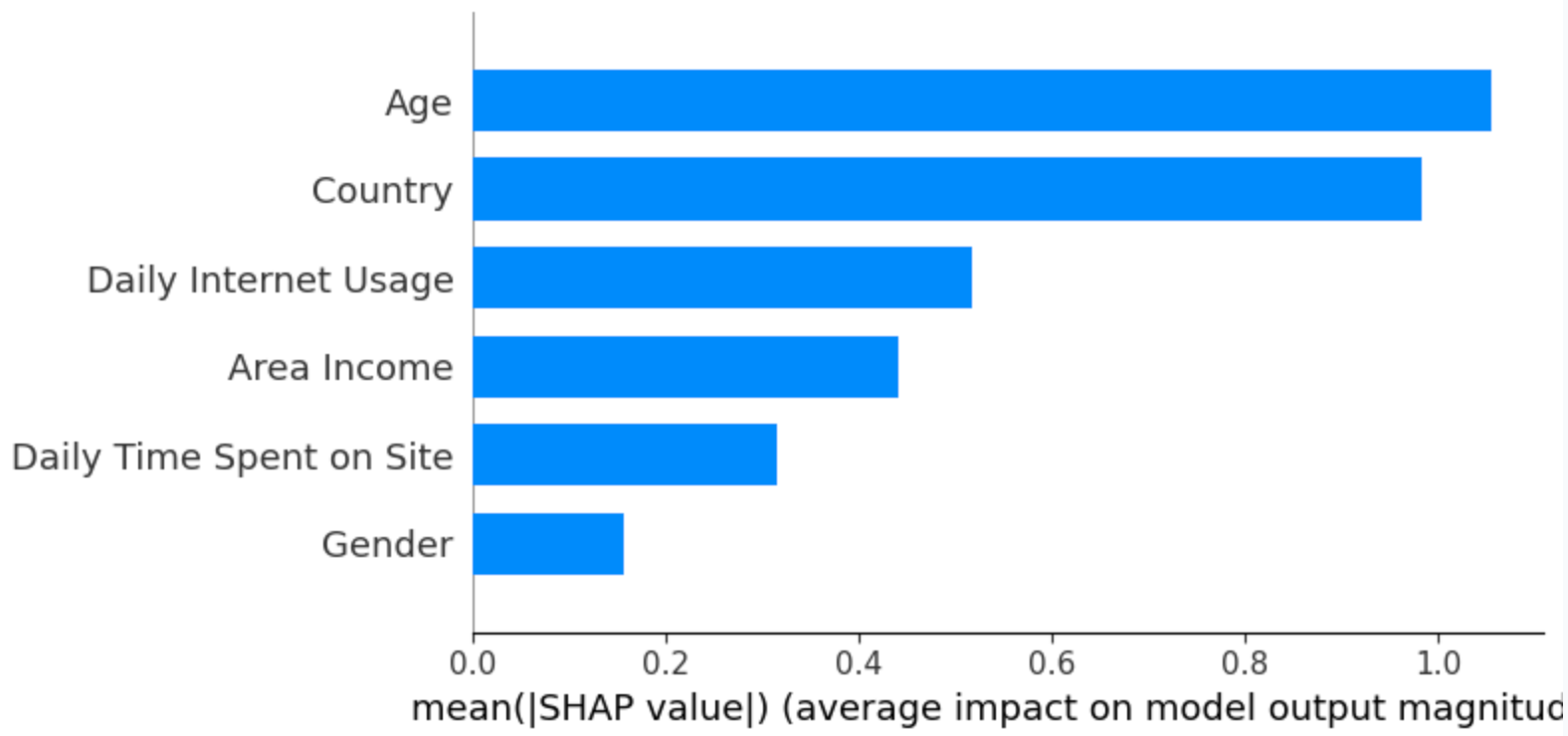
In the below plot
- The Y-axis represents the feature names arranged in descending order of importance, with the most important features at the top and the least important ones at the bottom
- The X-axis denotes the SHAP value, which serves as a measure of the extent of change in log odds
If we examine the "Age" feature and observe a notably positive value, it indicates that Age exerts a substantial positive influence on the output. In other words, when a person's age is higher, there is a heightened probability that the individual will be more inclined to click on the advertisement. Next, If we look at the feature “Daily Internet usage," we notice that it is mostly high with a negative SHAP value. It means high internet usage tends to negatively affect the output.
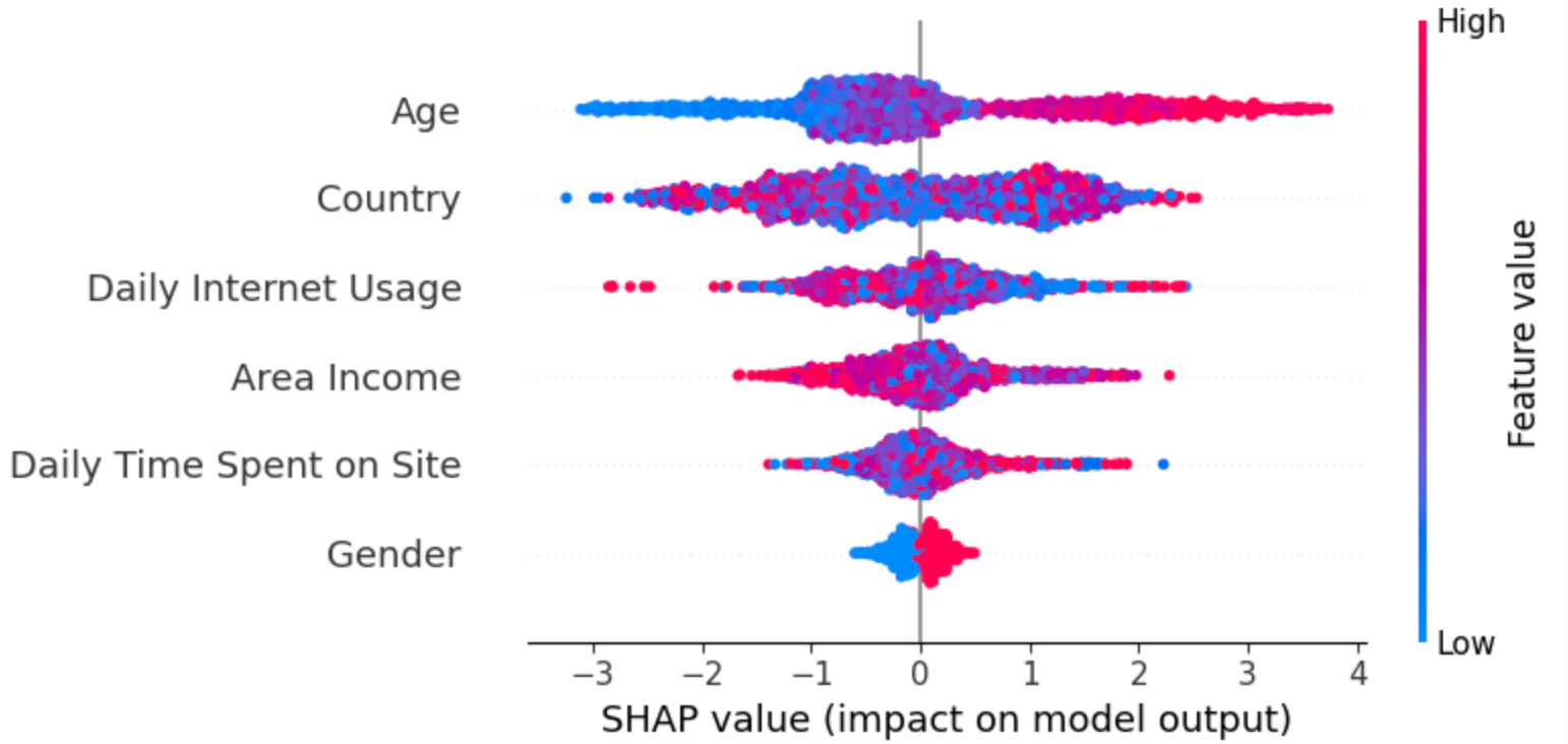
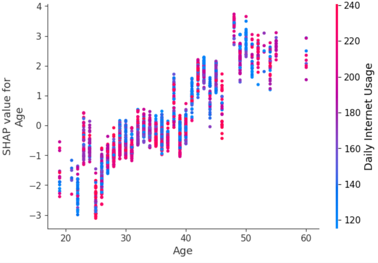
Let us now visualize the "dependence_plot" between the feature “Age” and “Daily Internet usage.” This suggests an interaction effect between Age and Internet Usage.
- Each dot is a single prediction from the dataset, the x-axis is the value of age,
- The y-axis is the SHAP value for that feature, which represents how much knowing that feature’s value changes the output of the model for that sample’s prediction. For this model the units are log-odds of clicking the ad.
- For example, a 60 year old with high internet usage is more likely to click on the ad.
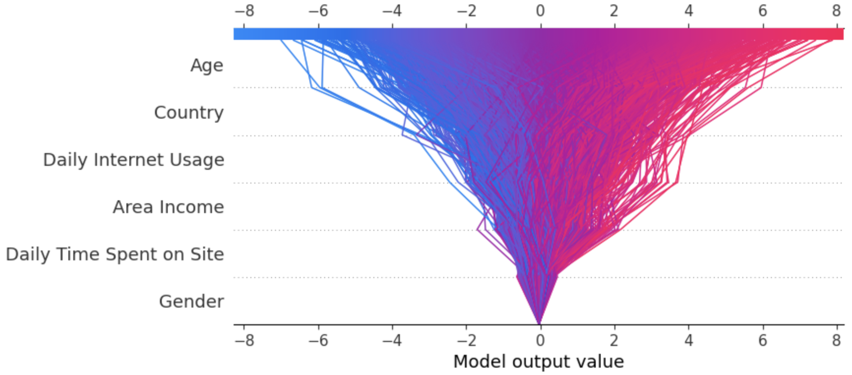
We will now look at the decision plot, the below code plots the decision plot.
expected_value = explainer.expected_value
shap.decision_plot(expected_value, shap_values, X_test)
Every line depicted on the decision plot illustrates the level of influence of individual features on a specific model prediction, thereby elucidating which feature values had the most impact on that prediction.
Saving and Loading XGBoost Models
Saving and Loading a trained model using the below code snippets.
model_new_hyper.save_model('model_new_hyper.model')
print("XGBoost model saved successfully.")
# Load the saved XGBoost model
import xgboost as xgb
loaded_model = xgb.Booster()
loaded_model.load_model('model_new_hyper.model')Now 'loaded_model' contains the trained XGBoost model, and can be used for predictions.
Disadvantages of XGBoost
XGBoost is a powerful and popular gradient boosting algorithm, It works by combining multiple decision trees to make a robust model. But this algorithm does have some disadvantages and limitations.
Complexity: An ensemble model, by nature, can be computationally demanding, and effectively tuning their hyperparameters necessitates extensive experimentation. Training an XGBoost model, especially when dealing with extensive datasets and numerous deep trees, can strain the computational resources, which might be a constraint on less capable hardware. In this article, we've already covered how this computational complexity can be mitigated through the use of GPUs.
Overfitting: XGBoost is sensitive to noisy data and outliers. While it has built-in regularization to handle overfitting, extreme cases of noise or outliers can still impact its performance. Also, it is a tree based model which can sometimes lead to overfitting.
Lack of Interpretability: Often XGBoost is called a "black box" model due to its lack of interpretability. We have shown how SHAP values and plots can be used to understand feature importance and impact on the model. However, when a large number of features are used to build the model, understanding the exact decision-making process of the model can be complex.
Memory Usage: Storing the model and its metadata can consume significant memory. Larger CPU instances (like the Paperspace C7) or GPU instances (like the A100 80G, if we are taking advantage of Paperspace’s powerful offerings)
Despite these disadvantages, XGBoost remains a robust and versatile algorithm in various Kaggle Competition, Machine Learning and data science tasks. Understanding these limitations and taking appropriate steps to mitigate them can help maximize the benefits of using XGBoost.
Conclusion
In this blog post, we have presented both the theoretical principles and practical aspects of the Gradient Boosting Algorithm. We provided a detailed overview of XGBoost, a scalable tree boosting system that is widely used by data scientists and provides state-of-the-art results on many problems. We've also included an extensive code demonstration where we implement XGBoost with the 'Ad Click-through Rate' dataset, using the Paperspace platform.
This tutorial outline provides a structured approach to learning and mastering XGBoost, covering everything from installation and data preparation to model training, evaluation, and deployment. We discussed a few disadvantages of the model and how to combat overfitting and underfitting. Also, we included SHAP plots to understand the important features of the model and interpret the model.
I hope that this article has provided a comprehensive understanding of XGBoost and inspired the readers to integrate it into practical machine learning scenarios to enhance predictive accuracy.