Gradient Boosting In Classification: Not a Black Box Anymore!

Machine learning algorithms require more than just fitting models and making predictions to improve accuracy. Most winning models in the industry or in competitions have been using Ensemble Techniques or Feature Engineering to perform better.

Ensemble techniques in particular have gained popularity because of their ease of use compared to Feature Engineering. There are multiple ensemble methods that have proven to increase accuracy when used with advanced machine learning algorithms. One such method is Gradient Boosting. While Gradient Boosting is often discussed as if it were a black box, in this article we'll unravel the secrets of Gradient Boosting step by step, intuitively and extensively, so you can really understand how it works.

In this article we'll cover the following topics:

• What Is Gradient Boosting?
• Gradient Boosting in Classification
  • An Intuitive Understanding: Visualizing Gradient Boosting
  • A Mathematical Understanding
• Implementation of Gradient Boosting in Python
• Comparing and Contrasting AdaBoost and Gradient Boost
• Advantages and Disadvantages of Gradient Boost
• Conclusion

What is Gradient Boosting?

Let's start by briefly reviewing ensemble learning. Like the name suggests, ensemble learning involves building a strong model by using a collection (or "ensemble") of "weaker" models. Gradient boosting falls under the category of boosting methods, which iteratively learn from each of the weak learners to build a strong model. It can optimize:

• Regression
• Classification
• Ranking

The scope of this article will be limited to classification in particular.

The idea behind boosting comes from the intuition that weak learners could be modified in order to become better. AdaBoost was the first boosting algorithm. AdaBoost and related algorithms were first cast in a statistical framework by Leo Breiman (1997), which laid the foundation for other researchers such as Jerome H. Friedman to modify this work into the development of the gradient boosting algorithm for regression. Subsequently, many researchers developed this boosting algorithm for many more fields of machine learning and statistics, far beyond the initial applications in regression and classification.

The term "Gradient" in Gradient Boosting refers to the fact that you have two or more derivatives of the same function (we'll cover this in more detail later on). Gradient Boosting is an iterative functional gradient algorithm, i.e an algorithm which minimizes a loss function by iteratively choosing a function that points towards the negative gradient; a weak hypothesis.

Gradient Boosting in Classification

Over the years, gradient boosting has found applications across various technical fields. The algorithm can look complicated at first, but in most cases we use only one predefined configuration for classification and one for regression, which can of course be modified based on your requirements. In this article we'll focus on Gradient Boosting for classification problems. We'll start with a look at how the algorithm works behind-the-scenes, intuitively and mathematically.

Gradient Boosting has three main components:

• Loss Function - The role of the loss function is to estimate how good the model is at making predictions with the given data. This could vary depending on the problem at hand. For example, if we're trying to predict the weight of a person depending on some input variables (a regression problem), then the loss function would be something that helps us find the difference between the predicted weights and the observed weights. On the other hand, if we're trying to categorize if a person will like a certain movie based on their personality, we'll require a loss function that helps us understand how accurate our model is at classifying people who did or didn't like certain movies.
• Weak Learner - A weak learner is one that classifies our data but does so poorly, perhaps no better than random guessing. In other words, it has a high error rate. These are typically decision trees (also called decision stumps, because they are less complicated than typical decision trees).
• Additive Model - This is the iterative and sequential approach of adding the trees (weak learners) one step at a time. After each iteration, we need to be closer to our final model. In other words, each iteration should reduce the value of our loss function.

An Intuitive Understanding: Visualizing Gradient Boost

Let's start with looking at one of the most common binary classification machine learning problems. It aims at predicting the fate of the passengers on Titanic based on a few features: their age, gender, etc. We will take only a subset of the dataset and choose certain columns, for convenience. Our dataset looks something like this:

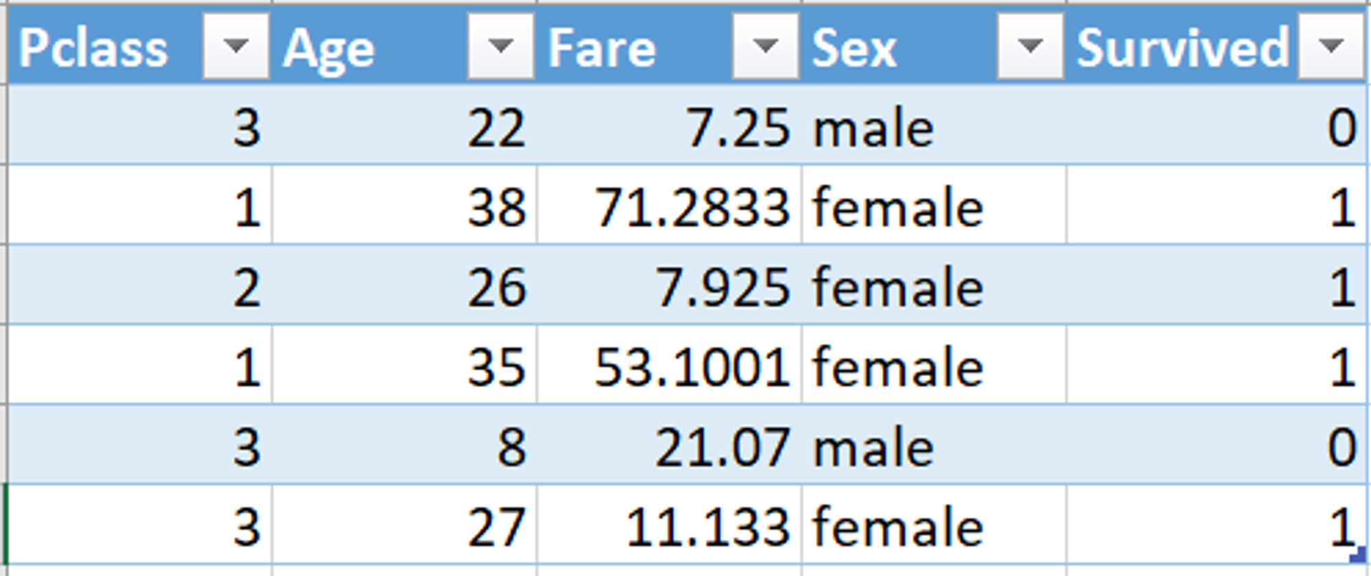
• Pclass, or Passenger Class, is categorical: 1, 2, or 3.
• Age is the age of the passenger when they were on the Titanic.
• Fare is the Passenger Fare.
• Sex is the gender of the person.
• Survived refers to whether or not the person survived the crash; 0 if they did not, 1 if they did.

Now let's look at how the Gradient Boosting algorithm solves this problem.

We start with one leaf node that predicts the initial value for every individual passenger. For a classification problem, it will be the log(odds) of the target value. log(odds) is the equivalent of average in a classification problem. Since four passengers in our case survived, and two did not survive, log(odds) that a passenger survived would be:

This becomes our initial leaf.

The easiest way to use the log(odds) for classification is to convert it to a probability. To do so, we'll use this formula:

Note: Please bear in mind that we have rounded off everything to one decimal place here, and hence the log(odds) and probability are the same, which may not be the case always.

If the probability of surviving is greater than 0.5, then we first classify everyone in the training dataset as survivors. (0.5 is a common threshold used for classification decisions made based on probability; note that the threshold can easily be taken as something else.)

Now we need to calculate the Pseudo Residual, i.e, the difference between the observed value and the predicted value. Let us draw the residuals on a graph.

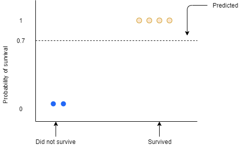
The blue and the yellow dots are the observed values. The blue dots are the passengers who did not survive with the probability of 0 and the yellow dots are the passengers who survived with a probability of 1. The dotted line here represents the predicted probability which is 0.7

We need to find the residual which would be :

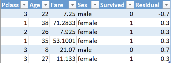
Here, 1 denotes Yes and 0 denotes No.

We will use this residual to get the next tree. It may seem absurd that we are considering the residual instead of the actual value, but we shall throw more light ahead.

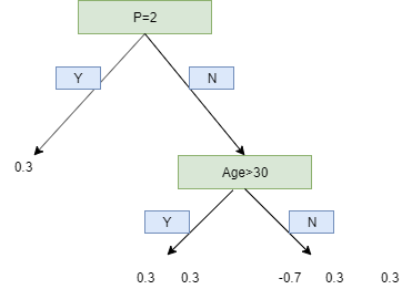
We use a limit of two leaves here to simplify our example, but in reality, Gradient Boost has a range between 8 leaves to 32 leaves.

Because of the limit on leaves, one leaf can have multiple values. Predictions are in terms of log(odds) but these leaves are derived from probability which cause disparity. So, we can't just add the single leaf we got earlier and this tree to get new predictions because they're derived from different sources. We have to use some kind of transformation. The most common form of transformation used in Gradient Boost for Classification is :

The numerator in this equation is sum of residuals in that particular leaf.

The denominator is sum of (previous prediction probability for each residual ) * (1 - same previous prediction probability).

The derivation of this formula shall be explained in the Mathematical section of this article.

For now, let us put the formula into practice:

The first leaf has only one residual value that is 0.3, and since this is the first tree, the previous probability will be the value from the initial leaf, thus, same for all residuals. Hence,

For the second leaf,

Similarly, for the last leaf:

Now the transformed tree looks like:

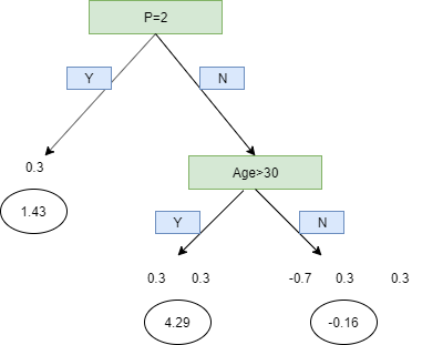
Now that we have transformed it, we can add our initial lead with our new tree with a learning rate.

Learning Rate is used to scale the contribution from the new tree. This results in a small step in the right direction of prediction. Empirical evidence has proven that taking lots of small steps in the right direction results in better prediction with a testing dataset i.e the dataset that the model has never seen as compared to the perfect prediction in 1st step. Learning Rate is usually a small number like 0.1

We can now calculate new log(odds) prediction and hence a new probability.

For example, for the first passenger, Old Tree = 0.7. Learning Rate which remains the same for all records is equal to 0.1 and by scaling the new tree, we find its value to be -0.16. Hence, substituting in the formula we get:

Similarly, we substitute and find the new log(odds) for each passenger and hence find the probability. Using the new probability, we will calculate the new residuals.

This process repeats until we have made the maximum number of trees specified or the residuals get super small.

A Mathematical Understanding

Now that we have understood how a Gradient Boosting Algorithm works on a classification problem, intuitively, it would be important to fill a lot of blanks that we had left in the previous section which can be done by understanding the process mathematically.

We shall go through each step, one at a time and try to understand them.

xi - This is the input variables that we feed into our model.

yi- This is the target variable that we are trying to predict.

We can predict the log likelihood of the data given the predicted probability

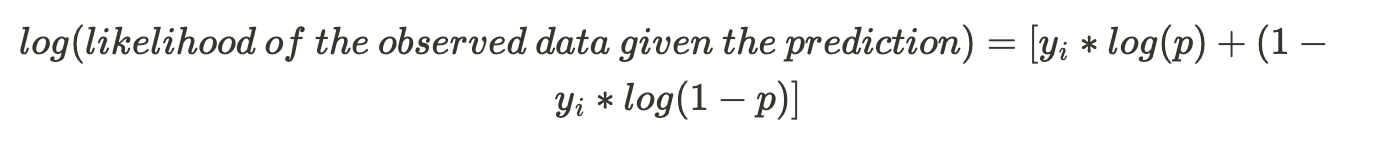
yi is observed value ( 0 or 1 ).

p is the predicted probability.

The goal would be to maximize the log likelihood function. Hence, if we use the log(likelihood) as our loss function where smaller values represent better fitting models then:

Now the log(likelihood) is a function of predicted probability p but we need it to be a function of predictive log(odds). So, let us try and convert the formula :

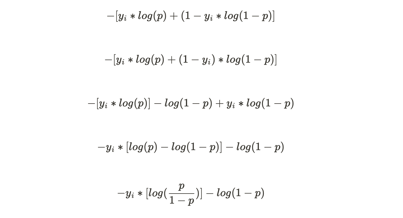
We know that :

Substituting,

Now,

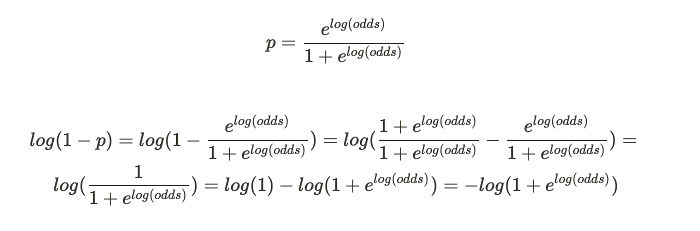
Hence,

Now that we have converted the p to log(odds), this becomes our Loss Function.

We have to show that this is differentiable.

This can also be written as :

Now we can proceed to the actual steps of the model building.

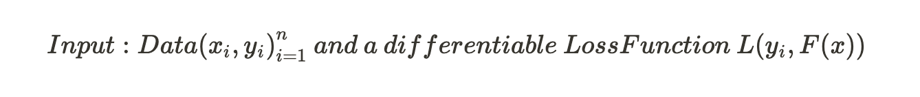
Step 1: Initialize model with a constant value

Here, yi is the observed values, L is the loss function, and gamma is the value for log(odds).

We are summating the loss function i.e. we add up the Loss Function for each observed value.

argmin over gamma means that we need to find a log(odds) value that minimizes this sum.

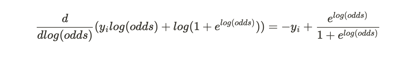
Then, we take the derivative of each loss function :

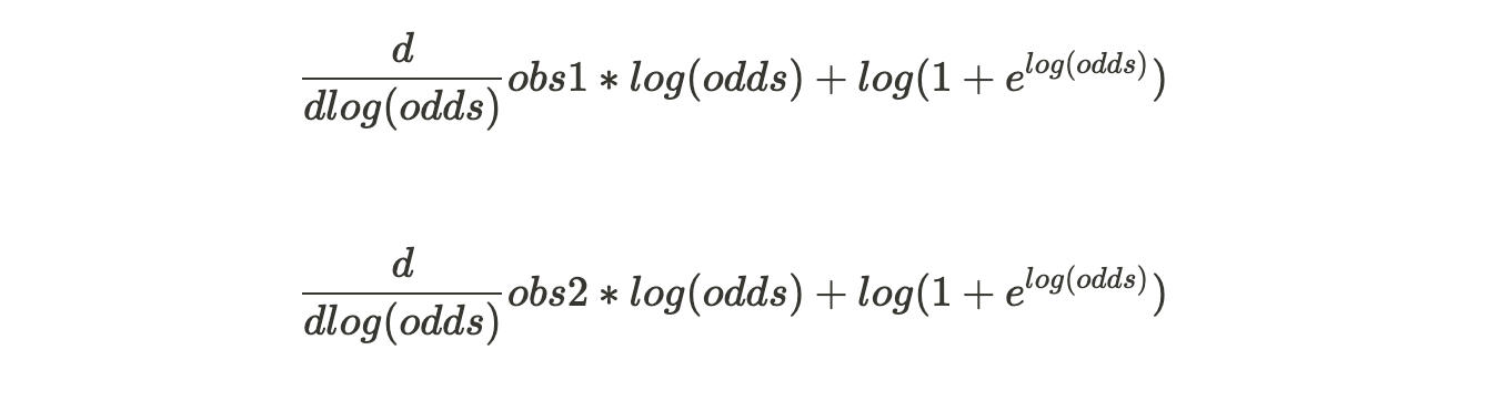
... and so on.

Step 2: for m = 1 to M:

(A)

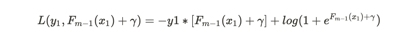
This step needs you to calculate the residual using the given formula. We have already found the Loss Function to be as :

Hence,

(B) Fit a regression tree to the residual values and create terminal regions

Because the leaves are limited for one branch hence, we might have more than one value in a particular terminal region.

In our first tree, m=1 and j will be the unique number for each terminal node. So R11, R21 and so on.

(C)

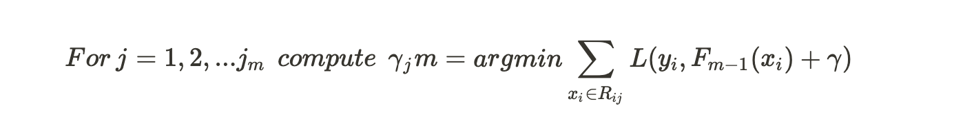
For each leaf in the new tree, we calculate gamma which is the output value. The summation should be only for those records which goes into making that leaf. In theory, we could find the derivative with respect to gamma to obtain the value of gamma but that could be extremely wearisome due to the hefty variables included in our loss function.

Substituting the loss function and i=1 in the equation above, we get:

We use second order Taylor Polynomial to approximate this Loss Function :

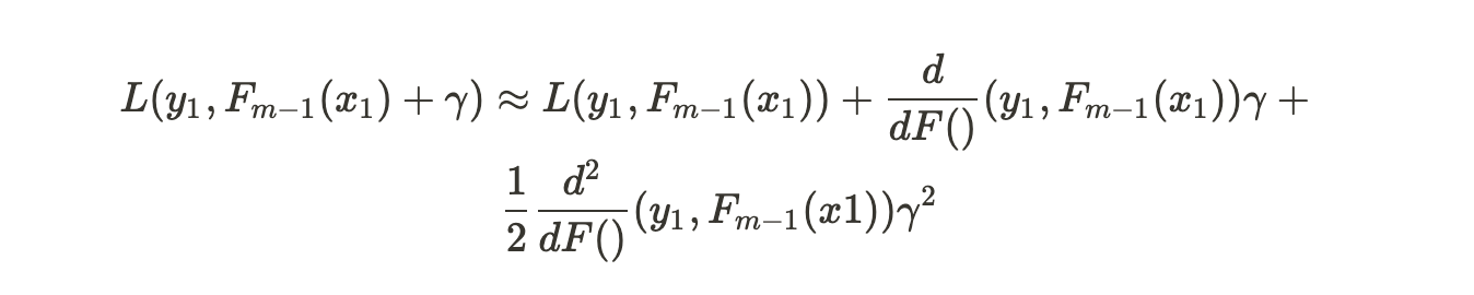
There are three terms in our approximation. Taking derivative with respect to gamma gives us:

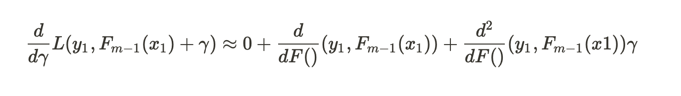
Equating this to 0 and subtracting the single derivative term from both the sides.

Then, gamma will be equal to :

The gamma equation may look humongous but in simple terms, it is :

We will just substitute the value of derivative of Loss Function

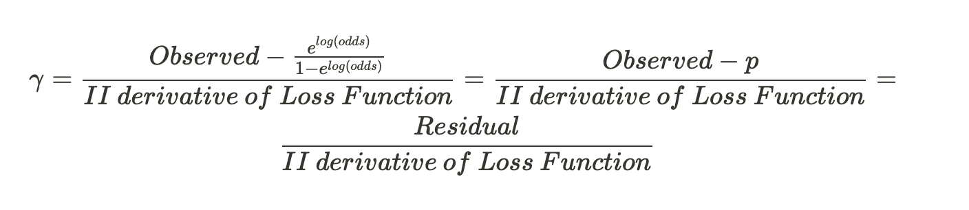
Now we shall solve for the second derivative of the Loss Function. After some heavy computations, we get :

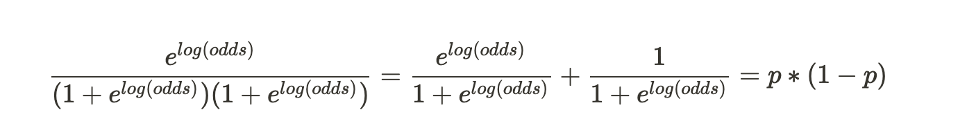
We have simplified the numerator as well as the denominator. The final gamma solution looks like :

We were trying to find the value of gamma that when added to the most recent predicted log(odds) minimizes our Loss Function. This gamma works when our terminal region has only one residual value and hence one predicted probability. But, do recall from our example above that because of the restricted leaves in Gradient Boosting, it is possible that one terminal region has many values. Then the generalized formula would be:

Hence, we have calculated the output values for each leaf in the tree.

(D)

This formula is asking us to update our predictions now. In the first pass, m =1 and we will substitute F0(x), the common prediction for all samples i.e. the initial leaf value plus nu, which is the learning rate into the output value from the tree we built, previously. The summation is for the cases where a single sample ends up in multiple leaves.

Now we will use this new F1(x) value to get new predictions for each sample.

The new predicted value should get us a little closer to actual value. It is to be noted that in contrary to one tree in our consideration, gradient boosting builds a lot of trees and M could be as large as 100 or more.

This completes our for loop in Step 2 and we are ready for the final step of Gradient Boosting.

Step 3: Output

If we get a new data, then we shall use this value to predict if the passenger survived or not. This would give us the log(odds) that the person survived. Plugging it into 'p' formula:

If the resultant value lies above our threshold then the person survived, else did not.

Implementation of Gradient Boosting using Python

We will work with the complete Titanic Dataset available in Kaggle. The dataset is already divided into training set and test set for our convenience.

The first step would be to import the libraries that we will need in the process.

import pandas as pd
from sklearn.ensemble import GradientBoostingClassifier
import numpy as np
from sklearn import metrics

Then we will load our training and testing data

train = pd.read_csv("train.csv")
test= pd.read_csv("test.csv")

Let us print out the datatypes of each column

train.info(), test.info()

<class 'pandas.core.frame.DataFrame'>
RangeIndex: 891 entries, 0 to 890
Data columns (total 12 columns):
PassengerId    891 non-null int64
Survived       891 non-null int64
Pclass         891 non-null int64
Name           891 non-null object
Sex            891 non-null object
Age            714 non-null float64
SibSp          891 non-null int64
Parch          891 non-null int64
Ticket         891 non-null object
Fare           891 non-null float64
Cabin          204 non-null object
Embarked       889 non-null object
dtypes: float64(2), int64(5), object(5)
memory usage: 83.6+ KB
<class 'pandas.core.frame.DataFrame'>
RangeIndex: 418 entries, 0 to 417
Data columns (total 11 columns):
PassengerId    418 non-null int64
Pclass         418 non-null int64
Name           418 non-null object
Sex            418 non-null object
Age            332 non-null float64
SibSp          418 non-null int64
Parch          418 non-null int64
Ticket         418 non-null object
Fare           417 non-null float64
Cabin          91 non-null object
Embarked       418 non-null object
dtypes: float64(2), int64(4), object(5)
memory usage: 36.0+ KB

Set PassengerID as our Index

# set "PassengerId" variable as index
train.set_index("PassengerId", inplace=True)
test.set_index("PassengerId", inplace=True)

We generate training target set and training input set and check the shape. All the variables except "Survived" columns becomes the input variables or features and the "Survived" column alone becomes our target variable because we are trying to predict based on the information of passengers if the passenger survived or not.

Join the train and test dataset to get a train_test dataset

train_test =  train.append(test)

Next step would be to preprocess the data before we feed it into our model.

We do the following preprocessing:

1. Remove columns "Name", "Age", "SibSp", "Ticket", "Cabin", "Parch".
2. Convert objects to numbers with pandas.get_dummies.
3. Fill nulls with a value of 0.0 and the most common occurrence in the case of categorical variable.
4. Transform data with MinMaxScaler() method.
5. Randomly split training set into train and validation subsets.

# delete columns that are not used as features for training and prediction
columns_to_drop = ["Name", "Age", "SibSp", "Ticket", "Cabin", "Parch"]
train_test.drop(labels=columns_to_drop, axis=1, inplace=True)

train_test_dummies = pd.get_dummies(train_test, columns=["Sex"])
train_test_dummies.shape

Check the missing values in the data:

train_test_dummies.isna().sum().sort_values(ascending=False)

Embarked      2
Fare          1
Sex_male      0
Sex_female    0
Pclass        0
dtype: int64

Let us handle these missing values. For "Embarked", we will impute the most occurring value and then create dummy variables, and for "Fare", we will impute 0.

train_test_dummies['Embarked'].value_counts()
train_test_dummies['Embarked'].fillna('S',inplace=True) # most common
train_test_dummies['Embarked_S'] = train_test_dummies['Embarked'].map(lambda i: 1 if i=='S' else 0)
train_test_dummies['Embarked_C'] = train_test_dummies['Embarked'].map(lambda i: 1 if i=='C' else 0)
train_test_dummies['Embarked_Q'] = train_test_dummies['Embarked'].map(lambda i: 1 if i=='Q' else 0)
train_test_dummies.drop(['Embarked'],axis=1,inplace=True)

train_test_dummies.fillna(value=0.0, inplace=True)

One final look to check if we have handled all the missing values.

train_test_dummies.isna().sum().sort_values(ascending=False)

Embarked_Q    0
Embarked_C    0
Embarked_S    0
Sex_male      0
Sex_female    0
Fare          0
Pclass        0
dtype: int64

All missing values seem to be handled.

Previously, we have generated our target set. Now we will generate our feature set/input set.

X_train = train_test_dummies.values[0:891]
X_test = train_test_dummies.values[891:]

It is time for one more final step before we fit our model, which would be to transform our data to get everything to one particular scale.

from sklearn.preprocessing import MinMaxScaler
scaler = MinMaxScaler()
X_train_scale = scaler.fit_transform(X_train)
X_test_scale = scaler.transform(X_test)

We have to now split our dataset into training and testing. Training to train our model and testing to check how good our model fits the dataset.

from sklearn.model_selection import train_test_split
X_train_sub, X_validation_sub, y_train_sub, y_validation_sub = train_test_split(X_train_scale, y_train, random_state=0)

Now we train our Gradient Boost Algorithm and check the accuracy at different learning rates ranging from 0 to 1.

learning_rates = [0.05, 0.1, 0.25, 0.5, 0.75, 1]
for learning_rate in learning_rates:
    gb = GradientBoostingClassifier(n_estimators=20, learning_rate = learning_rate, max_features=2, max_depth = 2, random_state = 0)
    gb.fit(X_train_sub, y_train_sub)
    print("Learning rate: ", learning_rate)
    print("Accuracy score (training): {0:.3f}".format(gb.score(X_train_sub, y_train_sub)))
    print("Accuracy score (validation): {0:.3f}".format(gb.score(X_validation_sub, y_validation_sub)))

('Learning rate: ', 0.05)
Accuracy score (training): 0.808
Accuracy score (validation): 0.834
('Learning rate: ', 0.1)
Accuracy score (training): 0.799
Accuracy score (validation): 0.803
('Learning rate: ', 0.25)
Accuracy score (training): 0.811
Accuracy score (validation): 0.803
('Learning rate: ', 0.5)
Accuracy score (training): 0.820
Accuracy score (validation): 0.794
('Learning rate: ', 0.75)
Accuracy score (training): 0.822
Accuracy score (validation): 0.803
('Learning rate: ', 1)
Accuracy score (training): 0.822
Accuracy score (validation): 0.816

This completes our code. A brief explanation about the parameters used here.

• n_estimators : The number of boosting stages to perform. Gradient boosting is fairly robust to over-fitting, so a large number usually results in a better performance.
• learning_rate : learning rate shrinks the contribution of each tree by learning_rate. There is a trade-off between learning_rate and n_estimators.
• max_features : The number of features to consider when looking for the best split.
• max_depth : maximum depth of the individual regression estimators. The maximum depth limits the number of nodes in the tree. Tune this parameter for best performance; the best value depends on the interaction of the input variables.
• random_state : random_state is the seed used by the random number generator.

Hyper tune these parameters to get the best accuracy.

Comparing and Contrasting AdaBoost and GradientBoost

Both AdaBoost and Gradient Boost learn sequentially from a weak set of learners. A strong learner is obtained from the additive model of these weak learners. The main focus here is to learn from the shortcomings at each step in the iteration.

AdaBoost requires users specify a set of weak learners (alternatively, it will randomly generate a set of weak learner before the real learning process). It increases the weights of the wrongly predicted instances and decreases the ones of the correctly predicted instances. The weak learner thus focuses more on the difficult instances. After being trained, the weak learner is added to the strong one according to its performance (so-called alpha weight). The higher it performs, the more it contributes to the strong learner.

On the other hand, gradient boosting doesn’t modify the sample distribution. Instead of training on a newly sampled distribution, the weak learner trains on the remaining errors of the strong learner. It is another way to give more importance to the difficult instances. At each iteration, the pseudo-residuals are computed and a weak learner is fitted to these pseudo-residuals. Then, the contribution of the weak learner to the strong one isn’t computed according to its performance on the newly distributed sample but using a gradient descent optimization process. The computed contribution is the one minimizing the overall error of the strong learner.

Adaboost is more about ‘voting weights’ and gradient boosting is more about ‘adding gradient optimization’.

Advantages and Disadvantages of Gradient Boost

Advantages of Gradient Boosting are:

• Often provides predictive accuracy that cannot be trumped.
• Lots of flexibility - can optimize on different loss functions and provides several hyper parameter tuning options that make the function fit very flexible.
• No data pre-processing required - often works great with categorical and numerical values as is.
• Handles missing data - imputation not required.

Pretty awesome, right? Let us look at some disadvantages too.

• Gradient Boosting Models will continue improving to minimize all errors. This can overemphasize outliers and cause overfitting.
• Computationally expensive - often require many trees (>1000) which can be time and memory exhaustive.
• The high flexibility results in many parameters that interact and influence heavily the behavior of the approach (number of iterations, tree depth, regularization parameters, etc.). This requires a large grid search during tuning.
• Less interpretative in nature, although this is easily addressed with various tools.

Conclusion

In this article, both the theoretical and the practical approach about the Gradient Boosting Algorithm have been proposed. Gradient Boosting has repeatedly proven to be one of the most powerful technique to build predictive models in both classification and regression. Because of the fact that Grading Boosting algorithms can easily overfit on a training data set, different constraints or regularization methods can be utilized to enhance the algorithm's performance and combat overfitting. Penalized learning, tree constraints, randomized sampling, and shrinkage can be utilized to combat overfitting.

Many of the real life machine learning challenges have been solved by Gradient Boosting.

Hope this article has encouraged you to explore Gradient Boosting in depth and start applying them into your real life machine-learning problems to boost your accuracy!

References

1. Gradient Boosting Classifiers in Python with Scikit-Learn
2. Boosting with AdaBoost and Gradient Boosting - The Making Of… a Data Scientist
3. Gradient Boost Part 1: Regression Main Ideas
4. Gradient Boosting Machines
5. Boosting with AdaBoost and Gradient Boosting - The Making Of… a Data Scientist
6. 3.2.4.3.6. sklearn.ensemble.GradientBoostingRegressor — scikit-learn 0.22.2 documentation
7. Gradient Boosting for Regression Problems With Example | Basics of Regression Algorithm
8. A Gentle Introduction to Gradient Boosting
9. Machine Learning Basics - Gradient Boosting & XGBoost
10. Understanding Gradient Boosting Machines