Gradient Boosted Trees and AutoML

Despite the popularity of deep learning, many AI teams have problems best solved by methods other than deep learning. This may be for reasons of interpretability, robustness of real-world data, regulatory requirements, available computing power or time, approved software, available expertise, or any number of other reasons.

In this project (and accompanying GitHub repository) we'll make use of gradient boosted decision trees (GBTs) to train a model and then deploy the model into production. Rather than apply deep learning techniques, we'll see that many ML problems can be addressed with a well-tuned GBT.

Our software of choice for this project is a state-of-the-art and open-source library called H2O. It includes advanced capabilities for GBT models, XGBoost models, and ensemble methods such as stacking via AutoML hyperparameter tuning.

Once the model is trained, we'll show how to use Gradient to deploy it into production as a REST API endpoint and send inference data to it.

In the accompanying GitHub repo we'll also show how to use Gradient Notebooks during the exploratory phase of a project as well as Gradient Workflows during the production phase.

Let's get to it!

Contents

• Data and Model
• Gradient Notebook
• Gradient Workflow
• Model deployment
• Conclusions
• Next steps

Accompanying Material

• ML Showcase
• GitHub repository

Data and Model

Our purpose in this project is to show end-to-end classical machine learning (rather than deep learning) on Gradient.

Since we want to solve a typical business problem well-suited to a method like GBT, we'll want tabular data with mixed datatypes rather than text or computer vision data.

We'll therefore be using the well-known UCI Census income dataset. A typical fragment of the data is shown below. Our goal will be to perform binary classification to predict whether a person's income is low or high. These are labeled <=50K and >50K respectively.

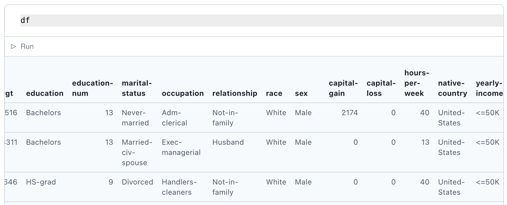
We see that the dataset consists of columns of demographic information of mixed data type: numerical, categorical, zeroes, etc. Luckily, decision trees tend to be robust for this type of data and we won't need preparation steps such as normalization or one-hot encoding.

Other details of the analysis are given in the sections below.

Gradient Notebook

Our goal within the Gradient Notebook will be to go from the initial raw dataset through to a saved model that is ready to be deployed.

H2O runs as a Java server, so we will initialize this from the notebook cell:

import h2o
h2o.init()

At larger scale, this allows it to run on a compute cluster as well as a single machine.

Since our data are small, we can import them as a CSV using the import method to H2O's data frame (similar to Pandas):

df = h2o.import_file(path = "income.csv")

Since Gradient Notebooks allow arbitrary Python code, other exploratory data analysis and preparation could be added here. We'll leave this out for now as it is not our focus and the model is performing correctly as is.

The data are separated into the feature columns x and a label column y, and are divided into non-overlapping random subsamples for training, validation, and testing. They are then passed to the model training.

We'll train the model using H2O's AutoML:

from h2o.automl import H2OAutoML
aml = H2OAutoML(max_models=20, seed=1)
aml.train(x=x, y=y, training_frame=train)

Despite its simplicity, AutoML is appropriate for many problems including usage by advanced users. This is because it searches a wide range of models and hyperparameters – comparable to and perhaps exceeding what an expert would search.

The dream of AutoML is that it can produce a model to provide sufficient business value in a fraction of the time that manual model tuning would take.

Nevertheless, AutoML does not solve every problem. In particular, many real business problems have business logic conditions or unusual metrics that may not be supported.

It is therefore important to note here that full manual tuning (and whatever other arbitrary code is needed) can be done in the same way as this project is done on Gradient. To manually tune the model we'd simply swap the AutoML bit with a manual tuning method such as H2OGradientBoostingEstimator.

Some of the models explored by AutoML include:

• Regular GBT (also known as GBM or gradient boosting machine)
• XGBoost model with grid of hyperparameter values
• A deep learning model
• Random forest
• Stacked ensembles of models (stacking = feed model output into next model input)

Somewhat surprisingly we do in fact include deep learning techniques here! Nevertheless the focus for the this project is classical ML so that's what we stick with.

The model that works best for this dataset is the stacked ensemble. This is a common outcome for many scenarios in which a well-tuned GBT benefits from model ensembling. While ensembling can increase accuracy, it can also increase compute time and reduce interpretability – so it ends up being useful only in certain situations.

Once training is done, a wealth of information is revealed. The model "leaderboard," for example, shows how various models are performing:

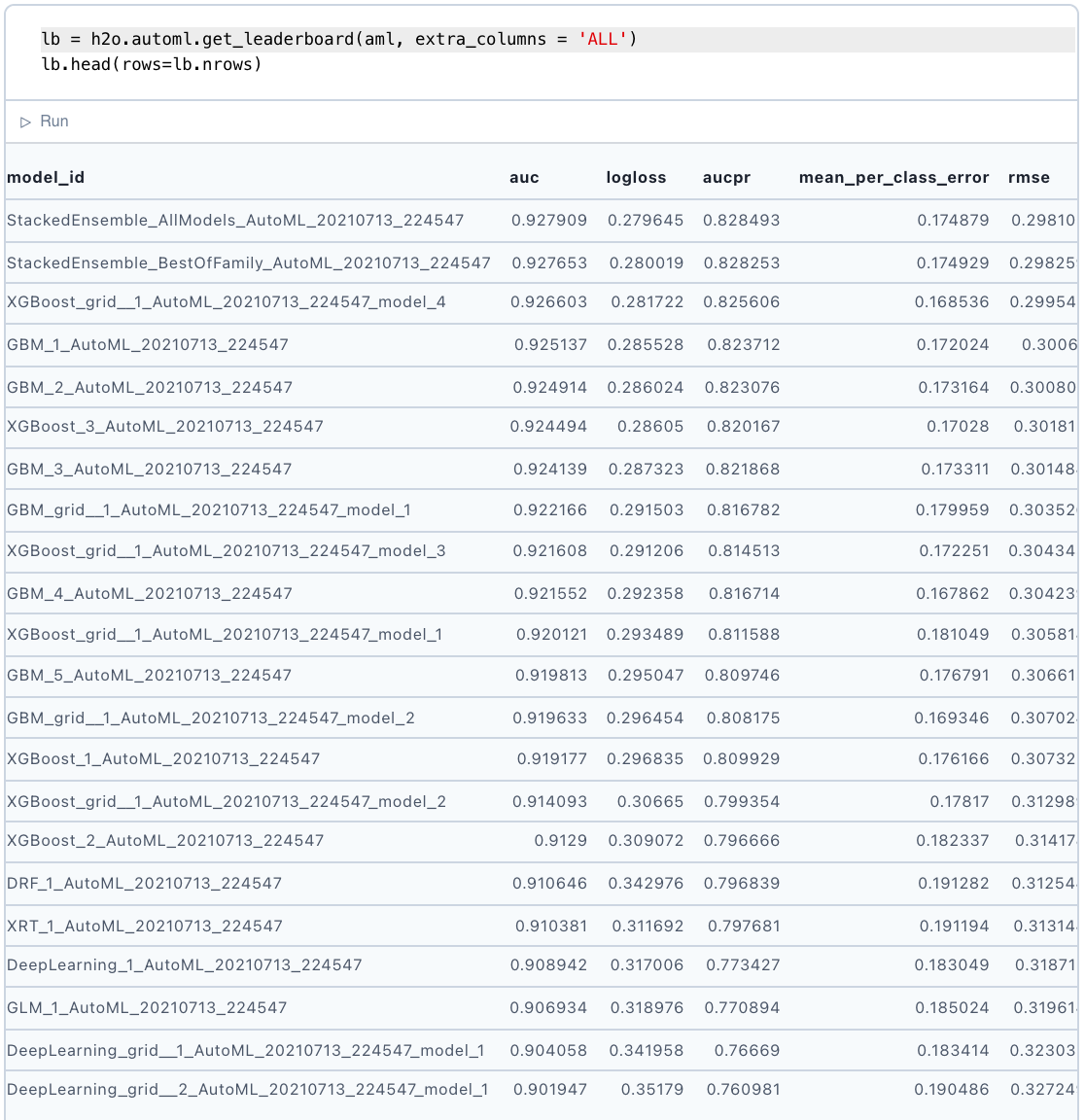
Model metrics are also available:

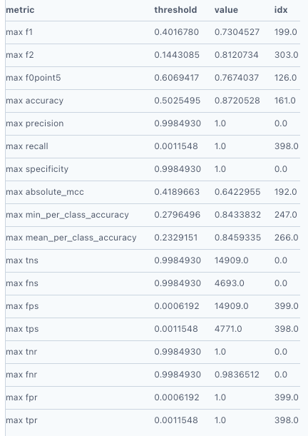
Here we used the default metric for binary classification: area under the curve, or AUC. This is the area encompassed by the plot of true positive rate versus false positive rate. The best possible value is 1 and here we get about 0.92 on the validation set, so the model appears to be performing well.

We might also see from the full leaderboard that the deep learning tasks took more than 20x as long as the other methods and performed worse. This is not necessarily a fair comparison as it is not extensively explored, yet nevertheless we see that for a quick analysis to solve the problem, classical ML was sufficient in this case.

H2O has recorded an abundance of information about the models, including metrics. Gradient has the ability to record these metrics during both experimentation and production. Metrics can be used as-are, or post-processed into something with greater business value such as expected revenue.

After training we can measure the performance of the model on the unseen testing data to check its generalization capability in the usual way.

Finally, we can save the model so that it is available for deployment into production. The get_genmodel argument outputs the h2o-genmodel.jar Java dependency that the model needs for deployment.

modelfile = model.download_mojo(path="/storage", get_genmodel_jar=True)

At Gradient's current state of development, it has integrations for model production with TensorFlow or ONNX. We therefore deploy the model directly using Java (see Model Deployment, below). We consider this of value to show because (1) end-to-end data science should include deployment to production and (2) this method is generic to any H2O model on Gradient, which encompasses most of what one would want to do with classical ML to solve business problems.

Gradient Workflow

Gradient's two main components are Notebooks and Workflows.

Notebooks are designed to help you get up and running quickly with data exploration, model experimentation, and access to hardware accelerators such as GPUs.

Workflows are designed to move a project into production using modern MLOps principles such as Git, Kubernetes, microservices, and YAML. Users do not require DevOps expertise to use Gradient as an orchestration platform.

In this project, we show how the analysis above can be done in both a Notebook as well as in a Workflow.

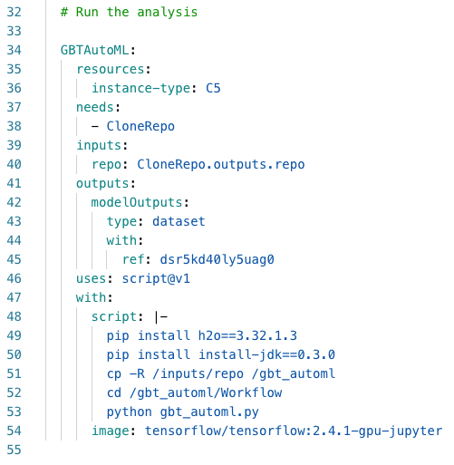
There is a Python .py script that is called by the YAML file that contains the specification of the Workflow. This gives a fully versioned description of the steps and the Python and YAML can be developed with no prejudice toward any particular IDE or environment.

The Workflow YAML specification looks like this:

The Workflow is run by invocation from the command line, with the following type of command:

gradient workflows run \
  --id         abc123de-f567-ghi8-90jk-l123mno456pq \
  --path       ./Workflow/gbt_automl.yaml \
  --apiKey     ab12cd34ef56gh78ij90kl12mn34op

The API can also be stored in your configuration instead of being given. In the future, Workflow invocation will be supported from the GUI and SDK. The Workflow and output datasets are visible in the GUI upon completion:

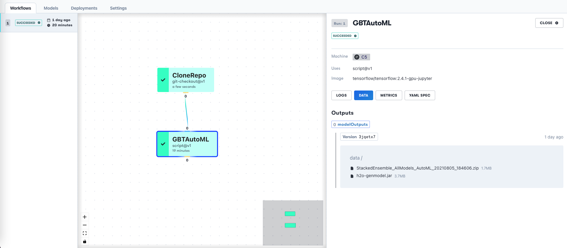
The Workflow is represented as a directed acyclic graph (DAG). Although this example is simple, it's straightforward to extend the steps, adding for example a separate data preparation job, multiple models, and so on.

We can also view other information from the Workflow such as previous runs and the versioned output dataset.

The output from the Workflow is the same as from the Notebook – a trained model that is ready to be deployed!

Model Deployment

One of Gradient's aims is to make model deployment as easy as possible even when hardware acceleration is present.

While there is quite extensive integration with TensorFlow for deep learning models, at present the H2O classical ML model here is deployed using Java. Nevertheless, this is valuable to show for the reasons mentioned above (end-to-end data science, and H2O/Java is very general), and Gradient's integrations will increase in the future as the project develops.

The setup is based upon the example in this blog entry by Spikelab, with several modifications.

The Notebook and/or Workflow project sections output an H2O model in MOJO (Model ObJect, Optimized). MOJO is the preferred format for saving models as it is portable and more general than POJO (Plain Old Java Object).

The model is named as follows:

StackedEnsemble_AllModels_AutoML_20210621_203855.zip

and there is a single associated Java dependency: h2o-genmodel.jar.

We use the simple web framework Javalin to build a Java project with Maven that contains the model (Model.java) and an app (App.java) that sets the model up as a REST endpoint.

We create the project using the command line within the Gradient container as opposed to using an IDE GUI such as IntelliJ or Eclipse. We also use a slightly newer version of H2O, 3.32.1.3.

The Java code is modified from the regression example online to our binary classification example. This is why we've changed the called classes and datatypes. We've changed the H2O artifactID from h2o-genmodel to h2o-genmodel-ext-xgboost to accommodate the XGBoost models. The inference data contains both categorical and numerical datatypes.

Details of how to deploy are in the project GitHub repo, but in the terminal on Gradient, the deployment is started via Java and listens on a port:

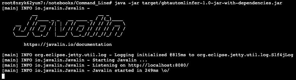
Inference data can be sent via curl. Here we submit a line of data from the income dataset and the model returns its response which is the predicted label for that row.

In this case, the person is predicted to be in the lower income class, <=50K.

Clearly this is not a full-scale enterprise production deployment, but let's take a look at what we're doing here. We have a model on a REST endpoint, inference data is being sent to it, and the model is returning responses.

Gradient has the infrastructure to scale this up and integrate with other tools such as model monitoring.

Conclusions

We have shown that Gradient is able to support advanced machine learning (ML) models outside of the subset of the field represented by deep learning. Which approach is best – deep learning or classical ML – is, as we've discovered, entirely situational.

This is what we did:

• We trained gradient boosted decision trees and other models using the well-known open source ML library H2O
• We used its AutoML automated machine learning functionality to search a number of model hyperparameter combinations and additional setups such as model ensembling via stacking
• We deployed the resulting model to production via Java as a REST endpoint

We used the following tools:

• We used a Gradient Notebook, which corresponds to the exploratory or experimental phase of a data science project
• We used a Gradient Workflow, which corresponds to a larger project that requires more rigor and production-grade practices

We then deployed on Gradient via the command line.

Next Steps

The end-to-end setup shown here in a Notebook, Workflow, and Deployment can be adapted for a wide range of business problems and other applications.

Here are some of the resources we mentioned during this tutorial:

• Project GitHub repository
• Project showcase
• Paperspace Gradient
• Gradient documentation
• Contact sales

And here are some additional links for further reading:

• H2O open source ML library
• H2O AutoML
• H2O MOJO model format
• Javalin web framework
• Spikelab blog entry with Java H2O deployment example
• UCI Census income dataset

Thanks for following along! Let us know if you have any questions or comments by reaching out!