
Bring this project to life
Activation functions are a common sight in deep learning architectures. In this article we will take a look at some of the common activation functions in deep learning applications as well as why they are used.
#  article dependencies
import torch
import torch.nn.functional as F
import numpy as np
import matplotlib.pyplot as plt
from tqdm.notebook import tqdm
from tqdm import tqdm as tqdm_regular
import seaborn as sns
Workings of a Neural Network
The whole idea/working principle behind neural networks is an ability to transform some kind of input data instance, be it a matrix or a vector, into a specific output representation of choice (scaler, vector or matrix). In order to do this, it essentially multiplies each element by specific numbers (weights) and passes them off as neurons in a new layer.
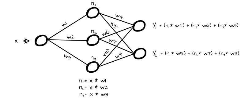
In order to do this effectively, the neural network must learn how neurons in one layer are related to the neurons of the next layer. When this is done from layer to layer we can then effectively learn a relationship between our input and output representations. Activation functions are what allow neural networks to learn this relationship between neurons.
Activation Functions
As stated in the previous section, activation functions aid neural networks in learning relationships between inputs and outputs by learning mappings from layer to layer. Activation functions can be split across a number of classes such as linear functions, binary step functions and non-linear functions.
Linear Activation Function
A linear activation function produces neurons which are proportional to their inputs. The simplest form of a linear activation function would be a case where neurons are not activated rather they are left as they are. Also called an identity function, this is synonymous to multiplying each neuron (x) by 1 in order to yield an activation y, hence y = x.
def linear_activation(values):
  """
  This function replicates the identity
  activation function
  """
  activations = [x for x in values]
  return activations


# generating values from -3 to 3
values = np.arange(-3, 4)

#  activating generated values
activations = linear_activation(values)
#  activations are the same as their original values
activations
>>>> [-3, -2, -1, 0, 1, 2, 3]

#  plotting activations
sns.lineplot(x=values, y=activations)
plt.xlabel('values')
plt.ylabel('activations')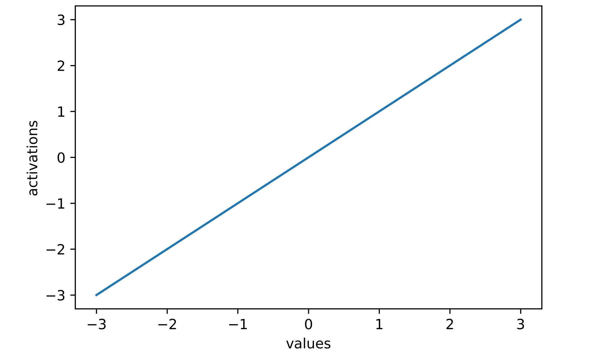
Binary Step Activation Functions
The binary step activation function defines a threshold for switching on or switching off neurons. It basically compares neuron values with the predefined threshold and only activates them if they are greater than or equal to the threshold value.
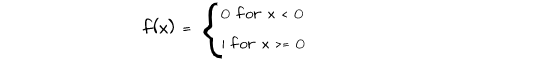
In the mathematical representation above, a threshold is set at zero such that any value below zero is assigned a value of 0 (not activated) and any value above zero is assigned a value of 1 (activated).
def binary_step_activation(values):
  """
  This function replicates the binary step
  activation function
  """
  activations = []

  for value in values:
    if value < 0:
      activations.append(0)
    else:
      activations.append(1)

  return activations


# generating values from -3 to 3
values = np.arange(-3, 4)

#  activating generated values
activations = binary_step_activation(values)
#  activations are zero for values less than zero
activations
>>>> [0, 0, 0, 1, 1, 1, 1]

#  plotting activations
sns.lineplot(x=values, y=activations, drawstyle='steps-post')
plt.xlabel('values')
plt.ylabel('activations')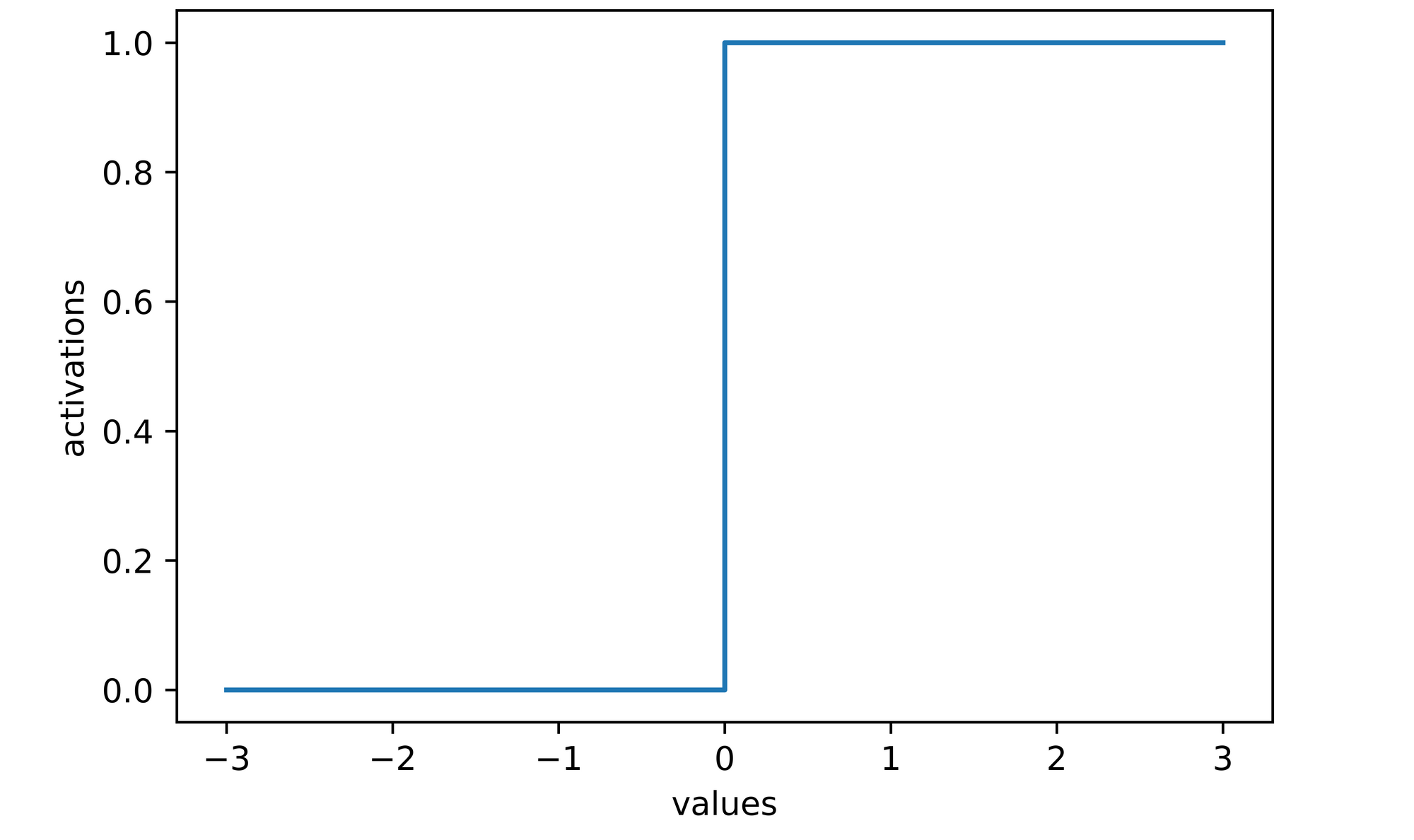
Non-Linear Activation Functions
By far the most widely used in deep learning applications, non-linear activation functions are the preferred choice in neural networks as they help the network to learn more complex relationships between inputs and outputs from layer to layer.
As evident from machine learning, a linear model (linear regression) is oftentimes not enough to effectively learn relationships in the context of a regression task which prompts the usage of a regularization parameter in a bid to try to learn more complex representations. Even at that, there is a limit to how well the linear model would fit.
The same applies in deep learning, most times there isn't a linear relationship between data instances commonly used for training deep learning models and their target representations. Think about it, could there realistically be a proportional relationship between several images of birds and whatever class label they are given? Very unlikely. What about an object detection task? It would be impossible for there to be a linear relationship between objects and the numerous pixels that could define their bounding boxes.
There is oftentimes a really complex relationship between inputs and targets in deep learning and non-linear activation functions help to transform neurons enough that the network is forced to learn a complex mapping from layer to layer. This section is dedicated to the commonly used non-linear activation functions in deep learning.
Bring this project to life
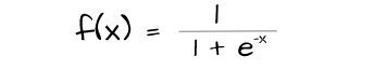
Sigmoid Function
Also known as the logistic function, the sigmoid function constrains values between the values 0 and 1. By doing this, it sort of presents a sort of probability which in turn represents the likelihood of each neuron's contribution to the values of the neurons in the next layer for that particular data instance.
However, due to the fact that neurons are constrained within a small scale sigmoid activation leads to the problem of varnishing gradient in deeper network architectures and is therefore mostly suitable for shallower architectures.
def sigmoid_activation(values):
  """
  This function replicates the sigmoid
  activation function
  """
  activations = []

  for value in values:
    activation = 1/(1 + np.exp((-1*value)))
    activations.append(activation)

  activations = [round(x, 3) for x in activations]
  return activations


#  generating values from -5 to 5
values = np.arange(-5, 6)

#  activating generated values
activations = sigmoid_activation(values)
#  all activations are now constrained between 0 and 1
activations
>>>> [0.01, 0.02, 0.05, 0.12, 0.27, 0.5, 0.73, 0.88, 0.95, 0.98, 0.99]

#  plotting activations
sns.lineplot(x=values, y=activations)
plt.xlabel('values')
plt.ylabel('activations')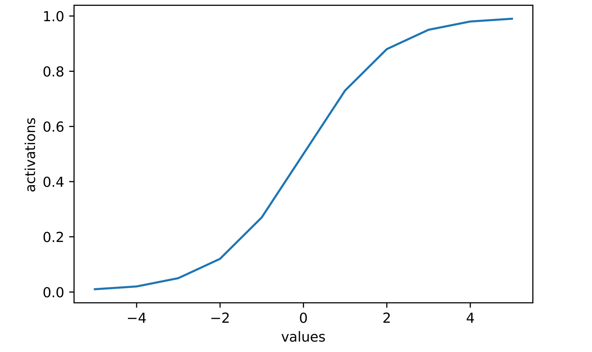
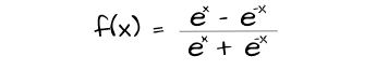
Hyperbolic Tangent Activation Function
Similarly to the sigmoid function the hyperbolic tangent function, commonly called the tanh activation function, constrains values not within 0 and 1 but within -1 and 1. It effectively regularizes the neurons in each layer.
This activation is seen as an improvement on the sigmoid activation functions as its activations are zero centered which is beneficial to gradient descent. However, just like the sigmoid, it is susceptible to varnishing gradient in deeper architectures as activations are constrained between a small scale as well.
def tanh_activation(values):
  """
  This function replicates the tanh
  activation function
  """
  activations = []

  for value in values:
    activation = (np.exp(value) - np.exp((-1*value)))/(np.exp(value) + np.exp((-1*value)))
    activations.append(activation)

  activations = [round(x, 2) for x in activations]
  return activations


#  generating values from -5 to 5
values = np.arange(-5, 6)

#  activating generated values
activations = tanh_activation(values)
#  all activations are now constrained between -1 and 1
activations
>>>> [-1.0, -1.0, -1.0, -0.96, -0.76, 0.0, 0.76, 0.96, 1.0, 1.0, 1.0]

#  plotting activations
sns.lineplot(x=values, y=activations)
plt.xlabel('values')
plt.ylabel('activations')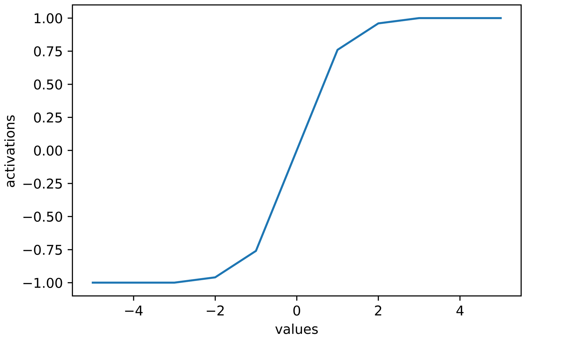
Rectified Linear Unit Activation Function (ReLU)
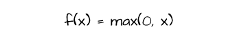
One of the most popular activation functions, the ReLU activation works by assigning a value of zero to any neuron with a negative value and leaves neurons with positive values untouched. It is represented mathematically as depicted below.
The ReLU activation is more computationally efficient in comparison to sigmoid and tanh, as negative neurons are zeroed thereby reducing computation. However, while using the ReLU activation function, one could encounter a problem termed dying ReLU. As the optimization process progresses neurons are casted to zero via ReLU activation, if a significant number of neurons become zero these neurons cannot be updated further if need be as their gradients will be zero. This leads to a part of the network effectively dying.
def relu_activation(values):
  """
  This function replicates the relu
  activation function
  """
  activations = []

  for value in values:
    activation = max(0, value)
    activations.append(activation)

  return activations


#  generating values from -5 to 5
values = np.arange(-5, 6)

#  activating generated values
activations = relu_activation(values)
#  all negative values are zeroed
activations
>>>> [0, 0, 0, 0, 0, 0, 1, 2, 3, 4, 5]

#  plotting activations
sns.lineplot(x=values, y=activations)
plt.xlabel('values')
plt.ylabel('activations')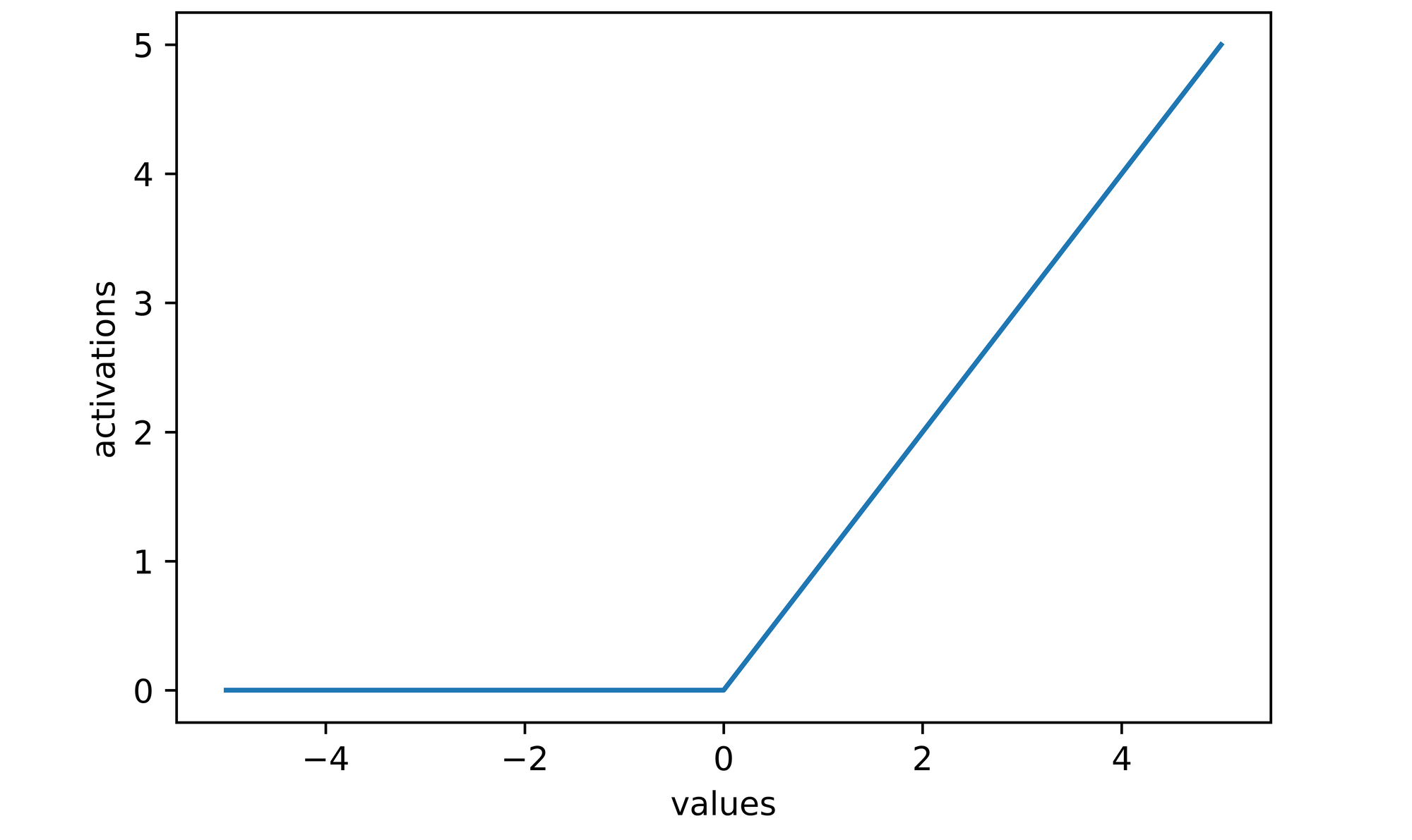
Leaky Rectified Linear Unit Activation Function (Leaky-ReLU)
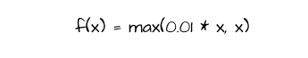
This activation function is a modified version of the ReLU function which attempts to solve the problem of dying ReLU. Unlike the ReLU function, leaky-ReLU does not cast non-positive values to zero rather it weights them by 0.01 such that they are insignificant enough however just alive so that they can be updated if the optimization process deems it necessary at any point during training.
def leaky_relu_activation(values):
  """
  This function replicates the leaky
  relu activation function
  """
  activations = []

  for value in values:
    activation = max(0.01*value, value)
    activations.append(activation)

  return activations


#  generating values from -5 to 5
values = np.arange(-5, 6)

#  activating generated values
activations = leaky_relu_activation(values)
#  negative values are not zeroed
activations
>>>> [-0.05, -0.04, -0.03, -0.02, -0.01, 0.0, 1, 2, 3, 4, 5]

#  plotting activations
sns.lineplot(x=values, y=activations)
plt.xlabel('values')
plt.ylabel('activations')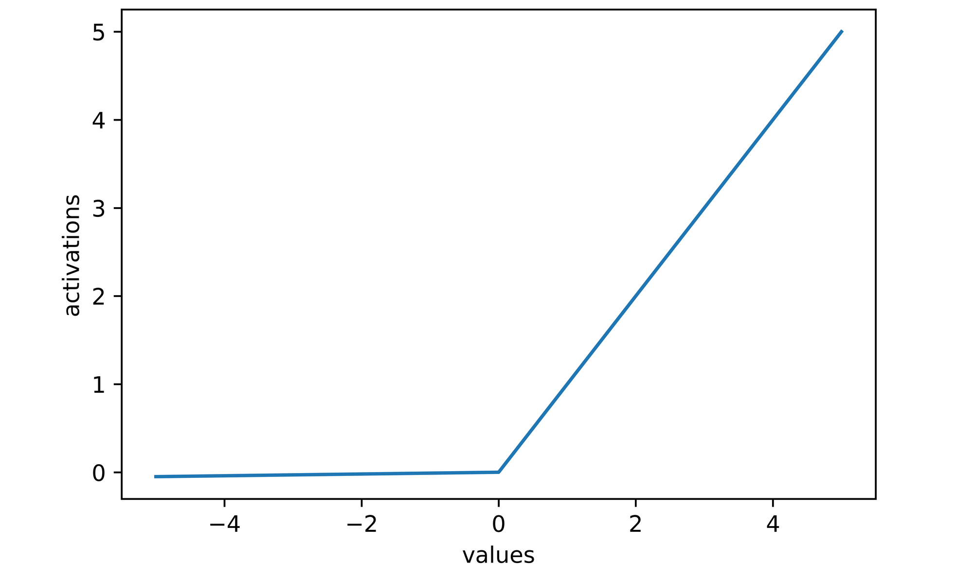
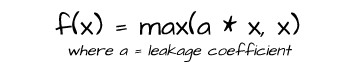
Parametric Rectified Linear Unit Activation Function
The Parametric Rectified Linear Unit (P-ReLU) activation function is quite similar to the leaky-ReLU function as it also tries to mitigate the problem of dying ReLU. However instead of specifying a constant weight for all negative values it instead designates the weight (leakage coefficient) as a learnable parameter which the neural network will be able to learn and optimize as a model is trained.
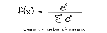
SoftMax Activation Function
The SoftMax activation function is one which is typically used in the output layer of neural networks designated to be used for multiclass classification tasks. It helps to produce the relative probabilities of the elements in the output vector. Unlike the sigmoid function, SoftMax takes the value of other elements in a representation into account when calculating probabilities hence the sum of all SoftMax activated values is always equal to one.
def softmax_activation(values):
  """
  This function replicates the softmax
  activation function
  """
  activations = []

  exponent_sum = sum([np.exp(x) for x in values])

  for value in values:
    activation = np.exp(value)/exponent_sum
    activations.append(activation)

  activations = [round(x, 3) for x in activations]

  return activations


#  generating values from -5 to 5
values = np.arange(-5, 6)

#  activating generated values using softmax
softmax_activations = softmax_activation(values)
#  values all sum up to 1
softmax_activations
>>>> [0.0, 0.0, 0.0, 0.001, 0.002, 0.004, 0.012, 0.031, 0.086, 0.233, 0.632]

#  activating generated values using sigmoid
sigmoid_activations = sigmoid_activation(values)
#  values do not sum up to 1
sigmoid_activations
>>>> [0.007, 0.018, 0.047, 0.119, 0.269, 0.5, 0.731, 0.881, 0.953, 0.982, 0.993]
Final Remarks
In this article we discussed about what activation functions are and why they are used in neural networks. We also took a look at several classes of activation functions concluding that non-linear activation functions are most suitable. Afterwards we touched on a number of common non-linear activation functions in theoretical, mathematical, graphical and code implementation terms.