Building on Squeeze-and-Excitation Networks (SENet) and the importance of Channel Attention, in this article we'll discuss ECA-Net: Efficient Channel Attention for Deep Convolutional Neural Networks published at CVPR 2020. The paper reinstates the importance of efficient channel attention and proposes a novel method which is a cheaper and better alternative to the popular Squeeze-and-Excitation networks (CVPR, TPAMI 2018).
This article is structured in four sections. Firstly, we will dive into the foundation of the paper and understand the importance of Cross Channel Interaction (CCI). We'll then discuss the design structure of ECA-Net and see how the design eliminates certain disadvantages of SENet. Afterwards we'll take a look at the results reported by the paper, and finally discuss some of the model's shortcomings.
You can run both ECA-Net and SENet for free on Gradient.
Table of Contents
- Local vs Neighborhood vs Global Information
- Cross-Channel Interaction (CCI)
- ECA-Net
- Adaptive Neighborhood Size
- Code
- Benchmarks
- Shortcomings
- References
Bring this project to life
The Tradeoff Between Local, Neighborhood, and Global Information

Before we dive into the paper, let's first understand the contextual importance of local information, neighborhood information, and global information. These will serve as the fundamental inspiration and justification for cross-channel interaction, which is the foundation for the Efficient Channel Attention (ECA-Net) structure proposed in the paper.
Imagine investigating the universe via a (hypothetically powerful) peephole, a telescope, and the naked eye. Each of the three options have different advantages and disadvantages, but in some cases the advantages of one option outweigh its disadvantages compared to the other options. Let's discuss in more detail.
The Telescope
Investigating space (basically the open, non-occluded sky) via a telescope is extremely informative, since it provides an enhanced view of faraway celestial objects. Let's take Saturn as an example. With the help of a powerful telescope, one can examine the rings of Saturn vividly and in fine detail. In this case, however, the field of view contains mainly just the rings; the body of Saturn itself is confined to the background. This can be thought of as showing the local information; your perspective is bounded within a finite local space, and while you perceive that information in sharp detail, it fails to include the larger context. Therefore, the advantage of the local information is that it pays more 'attention' to the fine details, although it fails to capture the contextual relationship on a larger scale, which would be important to perceive the scene as a whole. Think of it as the difference between a still life painting and a painting of a landscape. While the former is focused on fine local details of one thing (or view), the latter zooms out to show a larger scene, meanwhile sacrificing many smaller details.
The Peephole
Now imagine investigating Saturn through a (hypothetically powerful) peephole. Instead of just focusing on the rings, you'd have Saturn as a planet along with its rings in the field of view. Although you wouldn't be able to observe the finer details of the rings, you'll be able to see the planet completely. So you're sacrificing the luxury of perceiving the details of the rings to observe the celestial structure of Saturn. This would be defined as the neighborhood information, where Saturn and its rings are neighbors of each other, forming together a local contextual relationship. Note: this neighborhood does not provide global context of the scene, only context in the small area embedded within a larger scene.
The Naked Eye
Finally, imagine taking a moment to look into the bright night sky and find Saturn with your naked eye. Let's say you're able to see Saturn as a small, round, glowing sphere. Now you might have a better idea of the vast scale of the universe and how small Saturn is in it, as well as its location with respect to many other visible constellations. This is the global information. In this case you're sacrificing even more detail in order to have a better view of the full context. For instance, now you could map different relations between objects within the whole scene.
Another way of thinking of this is by differentiating between a micro image, a normal-scale image, and a panorama image. The micro image will include tiny details, the normal-scale image will provide local context, and the panorama will show the complete scene.
With this in mind, let's go over Cross Channel Interaction.
Cross-Channel Interaction (CCI)
Recall that a convolutional neural network is made up of convolutional layers with different numbers of learnable filters, which correspond to the number of channels in the output tensor from that respective layer. These tensors are 4-dimensional with shape (B, C, H, W), where B represents the batch size, C the number of channels (or total number of feature maps in that tensor, and thus also correlates to the total number of filters in the respective convolutional layer), while H and W represent the height and width of each feature map.
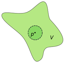
Assume that all the channels for a given tensor at any convolutional layer within the architecture are present within a finitely bounded space v, as shown in the above diagram. The context of the paper is to provide channel attention, and it aims to do so at a much cheaper complexity trade-off compared to Squeeze-and-Excitation Networks (SENet; this is a foundational paper in the domain of channel attention). Let's assume a small neighborhood within the global space v, and denote it as p. This neighborhood contains a finite subset of the whole set of channels. This forms the basis of cross channel interaction.
Recall that in SENet there are three modules which define the structure of the SE-block, including: (i) Squeeze module, (ii) Excitation module, and (iii) the Scaling module. The Squeeze module is responsible for reducing the spatial dimensionality of each feature map to singular pixels, or essentially unit points in the global space v shown above. Further, the Excitation module maps the whole global space v by a Fully Connected Multi-Layer Perceptron (FF-MLP) bottleneck containing a compression hidden layer with a reduction ratio r. This compression is the dimensionality reduction step. This is not optimal. Ideally one would want to map each channel to itself, thus obtaining global dependencies and relationships between each channel, however, this would be computationally very expensive which is why there exists a compression of the channels governed by the reduction ratio r. Below is a visualization of dimensionality reduction in the excitation module of a Squeeze-Excite block.
The Squeeze-and-Excitation network does incorporate Cross-Channel Interaction (CCI), which essentially means that the channels are not weighted and the channel attention is not learned for each channel in an isolated way. Instead, the weights for each channels are learned in respect to other channels. However, in SE-block, this CCI is also diluted with dimensionality reduction (DR) which is sub-optimal due to the complexity constraints. Thus, to address this, ECA-Net incorporates CCI without any DR by using local neighborhood problem shown in the first figure in the section denoted as p. So, ECA-Net obtains an adaptive local neighborhood size for each tensor and computes attention for each channel within that neighborhood p with respect to every other channel within that neighborhood p. We will later see how their method prevents dimensionality reduction (DR) and is cheaper than Squeeze-and-Excitation block.
ECA-Net
Based on our understanding of dimensionality reduction (DR) and Cross-Channel Interaction (CCI), let's now dissect the structure of ECA-Net. We will revisit the importance of cross-channel interaction and global information dependencies in a more math-y way in the next section.
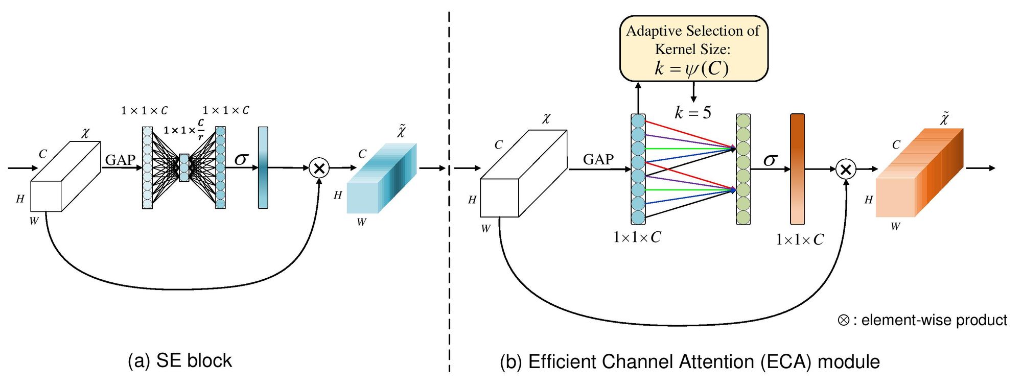
So, ECA-Net structure is extremely similar to that of SE-Net as shown in the above figure. Let's breakdown the individual components of the former. ECA-Net takes an input tensor which is the output of a convolutional layer and is 4-dimensional of the shape (B,C,H,W) where B represents the batch size, C represents the number of channels or total number of feature maps in that tensor and finally, H and W, represent the spatial dimensions of each feature map, namely, the height and width. The output of ECA block is also a 4-D tensor of the same shape. ECA-block is also made up of 3 modules which include:
- Global Feature Descriptor
- Adaptive Neighborhood Interaction
- Broadcasted Scaling
Let's take a look at each of them individually:
Global Feature Descriptor
As discussed in Squeeze-and-Excitation network, to address computational complexity of making the attention learning mechanism adaptive and dependent on each channel itself and since channels are each having H x W pixels, which makes a total of C x H x W information space, we use a global feature descriptor to reduce each feature map to a single pixel and thus reduce the space to just C x 1 x 1. This reduces complexity drastically and is able to capture encoded global information of each channels and thus make the channel attention adaptive and cheap at the same time. Both Squeeze-and-Excitation (SE) and Efficient Channel Attention (ECA) use the same global feature descriptor (named as the squeeze module in the SE-block) which is the Global Average Pooling (GAP). GAP takes the input tensor and reduces each feature maps to a single pixel by taking the average of all the pixels in that feature map.
Adaptive Neighborhood Interaction
As discussed in the previous section where we laid the foundation of this paper by describing Cross-Channel Interaction (CCI) in brief. So after the tensor is passed through GAP and is reduced to singular pixel space for each feature map, it is then subjected to an adaptive kernel which slides over this space with the kernel size describing the neighborhood size kept as adaptive. So in more detail, once we have the C x 1 x 1 tensor or C-length vector from GAP, it is subjected to a 1-D striding convolutional whose kernel size (k) is adaptive to the global channel space (C) and determined by the following formula:
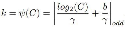
Thus, essentially k provides the size of the local neighborhood space which will be used to capture Cross-channel interaction while mapping the per-channel attention weights. In the above formula, b and γ are predefined hyper-parameters set to be 1 and 2 respectively. This function ψ(C) essentially approximates the closest odd number as the kernel size for the 1D convolutional based on the formula. Let's understand the rationale behind the formula:
From the understanding of group-wise convolutions which have been popularly adopted in convolutional neural network architectures, there exists an abstract mapping Φ between the number of channels C and the kernel size of the filters k. This mapping can be represented as: C = Φ(k). Thus the most simple relationship mapping would be that of a linear function which can be represented as Φ(k) = γ*k + b, however this would add severe limitations and might not be an accurate mapping. Since the inception of modern neural network designs, channels are usually set as different powers of 2. The reason behind this is that most buses in memory hardware are power of 2 based and thus you're not wasting any bits in the addressing mechanisms. So having channels in the order of powers of 2 maximizes performances and utilization of resources. This twitter thread contains more relevant discussion on the same. Thus, based on this, the authors introduce a non-linear mapping which can be defined as:
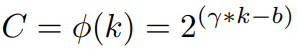
Solving for k in the above equation would give the ψ(C) described above. Thus, larger channel space will have a larger neighborhood size and vice versa.
Summarizing, the C x 1 x 1 tensor received post GAP is subjected to a striding 1D convolutional of kernel size k defined by the non-linear mapping adaptive to the total number of channels as per the function ψ(C). To note: This is a size depth preserving convolution, so the total number of channels in the output tensor post the 1D convolution as the same as total number of input channels - C. Thus, this eliminates by design the dimensionality reduction(DR) issue prevalent in Squeeze-and-Excitation module.
Broadcasted Scaling
After the weighted tensor of shape C x 1 x 1 is received from the 1D-convolution, it's simply passed through a sigmoid activation layer which thresholds each channel weights between the range of 0 to 1. This channel attention vector is then broadcasted to the input tensor size (C x H x W) and then element wise multiplied with it.
Therefore, summarizing, in ECA-block, the input tensor is first decomposed to a channel vector by passing through a Global Average Pooling layer followed by a 1D convolution with an adaptive kernel size and then passed through a sigmoid before being broadcasted and element wise multiplied with the input tensor. Thus, as compared to Squeeze-and-Excitation, ECA-Net is extremely cheap since the total number of parameters added is just k.
Let's compare ECA-Net with other attention mechanisms in terms of their properties and computational complexity overhead:
| Attention Mechanisms | DR | CCI | Parameter Overhead | Efficient |
|---|---|---|---|---|
| SE | Yes | Yes | 2C2/r | No |
| CBAM | Yes | Yes | 2C2/r + 2k2 | No |
| BAM | Yes | Yes | C/r(3C + 2C2/r + 1) | No (however the block integration strategy makes it cheap in terms of overhead) |
| GC | Yes | Yes | 2C2/r + C | No |
| GE-θ- | No | No | - | Yes |
| GE-θ | No | No | - | No |
| GE-θ+ | Yes | Yes | - | No |
| A2-Nets | Yes | Yes | - | No |
| GSoP-Nets | Yes | Yes | - | No |
| ECANet | No | Yes | k = 3 | Yes |
Note: DR = No and CCI = Yes are optimal and ideal. C represents the total number of channels and r represents the reduction ratio. The parameter overhead is per attention block.
Although the kernel size in ECA-block is defined by the adaptive function ψ(C), the authors throughout all experiments fixed the kernel size k to be 3. The reason behind this is not clear and hasn't been accurately addressed by the authors when this concern was raised by GitHub users on their official code repository in this issue.
Adaptive Neighborhood Size
As discussed in previous section where we emphasized on Cross-Channel Interaction (CCI) as the fundamental concept in Efficient Channel Attention (ECA) block. In this section we will understand how the authors reached the conclusion that CCI is important and the mathematical understanding behind the same.
Let's recap, in case of Squeeze-and-Excitation module, we have a Fully Connected Multi-Layer Perceptron (FC-MLP) where there is an input layer, hidden layer and output layer. The input layer has C neurons, the hidden layer C/r neurons and the output layer C neurons. This involves dimensionality reduction (DR) because of the reduction ratio r which makes the relationship mapping between channels to be indirect and thus non-optimal. The authors, thus, to investigate, first construct three different variants of Squeeze-and-Excitation block which doesn't involve dimensionality reduction. The name these three variants as: (i) SE-Var1, (ii) SE-Var2, and, (iii) SE-Var3 respectively.
SE-Var1 contains no parameter overhead and essentially computes the Global Average Pooling (GAP) of the input vector and then passes it through a sigmoid activation before broadcasting and element wise multiplying it with the input tensor. In equation form this can be represented as: σ(y) where y is the GAP(input) and σ is the Sigmoid activation.
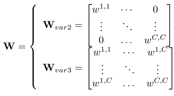
SE-Var2 is essentially a 1-to-1 connected network, thus contains one weight per channel and doesn't incorporate cross-channel interaction. Thus, the parameter overhead is the total number of channels C in the input tensor. In equation form, this can be represented as: σ(w ⊙ y) where w is the weights for each channels in the GAP vector denoted by y.
SE-Var3 is the holy grail of channel attention, where it has global cross-channel interaction and no dimensionality reduction. Essentially, this contains a fully connected no bottleneck reduction network to construct the channel attention weights. In equation form this can be represented as: σ(Wy) where W is the complete C x C weight matrix. However, although this is the optimal approach, this adds huge parameters (CxC more parameters to be precise) and computational complexity overhead.
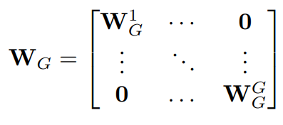
Essentially, SE-Var2 is the diagonal matrix of the complete C x C matrix and both weight matrices for SE-Var2 and SE-Var3 can be represented in the following matrix form:
Based on these three different variants, the authors design the construct of ECA-block where the weight matrix is constrained to a smaller neighborhood size than the whole C channels. Thus, based on the importance of CCI, the authors define this constraint to be G and it can be represented in matrix form as:
Here, the channels are divided into G groups where each group contains C/G channels and then they construct a SE-Var2 diagonal weight matrix within this group G. Thus the parameter overhead here is G which is also denoted formally as k as discussed in the earlier sections where the size of G is defined by the adaptive function ψ(C). And these G weights are shared across all strides of the 1D convolution and thus can be mathematically represented as: σ(C1Dk(y))
The authors perform ablation studies to observe the performance of each SE variant and compared it to the performance of ECA-block and as shown in the table below, ECA-block performs the best with the least parameter overhead. The authors also confirm the importance of channel attention because of the incremental performance obtained by SE-Var1 which contains no learnable parameters.
| Methods | Attention | Parameter Overhead | Top-1 Accuracy | Top-5 Accuracy |
|---|---|---|---|---|
| Vanilla | N/A | 0 | 75.20 | 92.25 |
| SE | σ(f{W1,W2}(y)) | 2 × C2/r | 76.71 | 93.38 |
| SE-Var1 | σ(y) | 0 | 76.00 | 92.90 |
| SE-Var2 | σ(w ⊙ y) | C | 77.07 | 93.31 |
| SE-Var3 | σ(Wy) | C2 | 77.42 | 93.64 |
| ECA | σ(C1Dk(y)) | k = 3 | 77.43 | 93.65 |
Code
Now, let's take a look at the snippet of ECA-block in PyTorch and Tensorflow:
PyTorch
### Import necessary dependencies
import torch
from torch import nn

class ECA(nn.Module):
    """Constructs a ECA module.
    Args:
        channel: Number of channels of the input feature map
    """

    def __init__(self, channel, k_size=3):
        super(ECA, self).__init__()
        self.avg_pool = nn.AdaptiveAvgPool2d(1)
        self.conv = nn.Conv1d(1, 1, kernel_size=k_size, padding=(k_size - 1) // 2, bias=False)

    def forward(self, x):
        # feature descriptor on the global spatial information
        y = self.avg_pool(x)

        # Two different branches of ECA module
        y = self.conv(y.squeeze(-1).transpose(-1, -2)).transpose(-1, -2).unsqueeze(-1)

        # Multi-scale information fusion
        y = torch.sigmoid(y)

        return x * y.expand_as(x)
TensorFlow
### Import necessary packages
import tensorflow as tf
def ECA(self, x):
k_size = 3
squeeze = tf.reduce_mean(x,[2,3],keep_dims=False)
squeeze = tf.expand_dims(squeeze, axis=1)
attn = tf.layers.Conv1D(filters=1,
kernel_size=k_size,
padding='same',
kernel_initializer=conv_kernel_initializer(),
use_bias=False,
data_format=self._data_format)(squeeze)
attn = tf.expand_dims(tf.transpose(attn, [0, 2, 1]), 3)
attn = tf.math.sigmoid(attn)
scale = x * attn
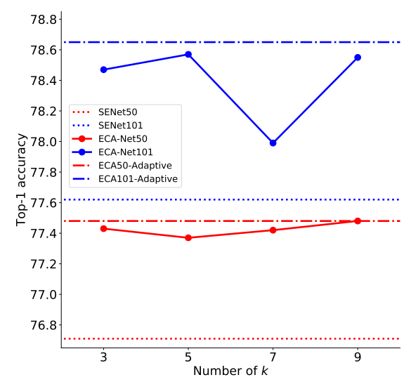
return x * attnAs discussed earlier, the authors do not use the adaptive kernel size defined by ψ(C) but rather set it to a default value of 3. Although the authors in their paper show the following graph suggesting their results to be based off an adaptive kernel size rather than a default of 3, however, a kernel size of 3 would result in the lowest parametric overhead.
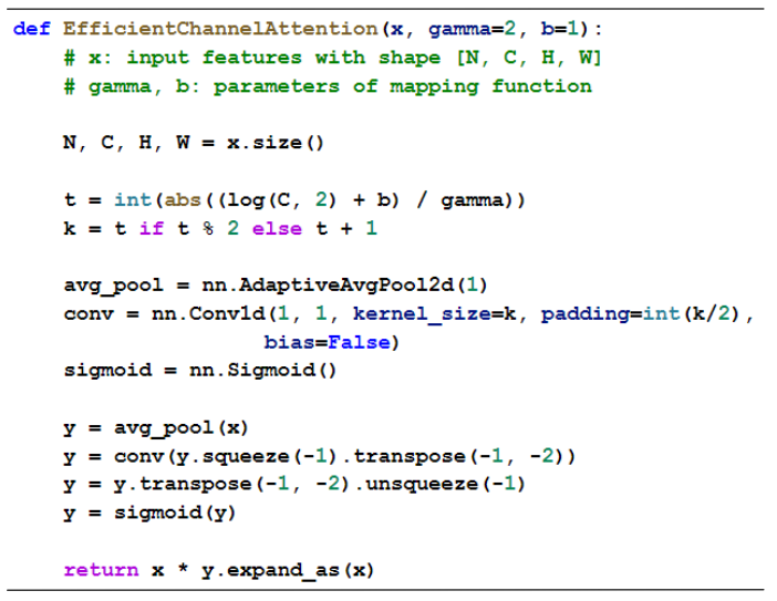
Additionally, as per the paper, the authors provide a PyTorch code snippet of ECA-block containing the adaptive function ψ(C) for computing the kernel size:
Benchmarks
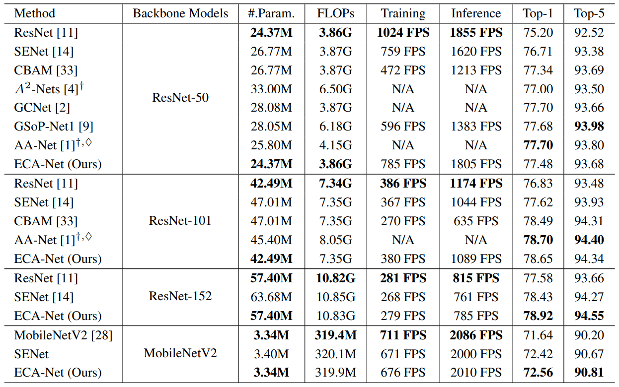
Here, we will go through the results the authors demonstrate for ECA-Net in different tasks starting from ImageNet-1k classification, object detection on MS-COCO and Instance segmentation on MS-COCO. The authors also provide additional metric of comparison like that of inference and training FPS (Frames per Second) which solidifies the efficiency of ECA-block attention as compared to other standard attention mechanisms popularly used in deep convolutional neural networks.
ImageNet-1k
Comparison of ECA-Net with other state of the art (SOTA) models:
The authors compare their ECA-Net models to other similar complexity models to demonstrate the efficiency of ECA-Net as shown in the following table:
| CNN Models | Parameters | FLOPs | Top-1 Accuracy | Top-5 Accuracy |
|---|---|---|---|---|
| ResNet-200 | 74.45M | 14.10G | 78.20 | 94.00 |
| Inception-v3 | 25.90M | 5.36G | 77.45 | 93.56 |
| ResNeXt-101 | 46.66M | 7.53G | 78.80 | 94.40 |
| DenseNet-264 (k=32) | 31.79M | 5.52G | 77.85 | 93.78 |
| DenseNet-161 (k=48) | 27.35M | 7.34G | 77.65 | 93.80 |
| ECA-Net50 | 24.37M | 3.86G | 77.48 | 93.68 |
| ECA-Net101 | 42.49M | 7.35G | 78.65 | 94.34 |
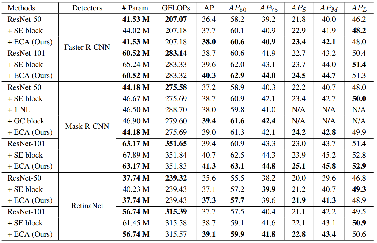
Object Detection on MS-COCO
Instance Segmentation on MS-COCO
| Methods | AP | AP50 | AP75 | APS | APM | APL |
|---|---|---|---|---|---|---|
| ResNet-50 | 34.1 | 55.5 | 36.2 | 16.1 | 36.7 | 50.0 |
| + SE block | 35.4 | 57.4 | 37.8 | 17.1 | 38.6 | 51.8 |
| + 1 NL | 34.7 | 56.7 | 36.6 | N/A | N/A | N/A |
| + GC block | 35.7 | 58.4 | 37.6 | N/A | N/A | N/A |
| + ECA (Ours) | 35.6 | 58.1 | 37.7 | 17.6 | 39.0 | 51.8 |
| ResNet-101 | 35.9 | 57.7 | 38.4 | 16.8 | 39.1 | 53.6 |
| + SE block | 36.8 | 59.3 | 39.2 | 17.2 | 40.3 | 53.6 |
| + ECA (Ours) | 37.4 | 59.9 | 39.8 | 18.1 | 41.1 | 54.1 |
Note- The authors used Mask R-CNN for this experiment
Although GC block performs superior than ECA block, however, GC is much more costlier in terms of computational complexity than ECA which justifies ECA performance.
Shortcomings
Although the papers propose a cheaper and more efficient way of computing Channel Attention as compared to Squeeze-and-Excitation, it does have it's fair share of drawbacks:
- As with every channel attention variant, ECA-Net also suffers from the curse of intermediate tensors which are broadcasted to the full shape of the input in the form of (C x H x W) and thus results in increased memory usage.
- As with every stand-alone channel attention variant, the block doesn't provide any form of per-pixel/ pixel-wise attention or essentially Spatial attention which is important in its own rights.
- The authors haven't provided a clear intuition behind the adaptive kernel size function ψ(C), especially the reason behind the default values of γ and b. The authors also haven't clarified of setting the kernel size as default 3 rather than using the adaptive function.