Autoencoders and Visual Similarity

Ever wondered how image search works, or how social media platforms are able to recommend similar images to those that you often like? In this article, we will be taking a look at another beneficial use of autoencoders, and attempting to explain their utility in computer vision recommendation systems.

Setup

We first need to import the relevant packages for the task today:

#  article dependencies
import torch
import torch.nn as nn
import torch.nn.functional as F
import torchvision
import torchvision.transforms as transforms
import torchvision.datasets as Datasets
from torch.utils.data import Dataset, DataLoader
import numpy as np
import matplotlib.pyplot as plt
import cv2
from tqdm.notebook import tqdm
from tqdm import tqdm as tqdm_regular
import seaborn as sns
from torchvision.utils import make_grid
import random
import pandas as pd

We also check the machine for a GPU, and enable Torch to run on CUDA if one is available.

#  configuring device
if torch.cuda.is_available():
  device = torch.device('cuda:0')
  print('Running on the GPU')
else:
  device = torch.device('cpu')
  print('Running on the CPU')

Visual Similarity

In the context of human vision, we humans are able to make comparison between images by perceiving their shapes and colors, using this information to access how similar they may be. However, when it comes to computer vision, in order to make sense of images their features have to be extracted first. Thereafter, in order to compare how similar two images may be, their features need to be compared in some kind of way so as to measure similarity in numerical terms.

The Role of Autoencoders

As we know, autoencoders are fantastic at representation learning. In fact, they learn representations well enough to be able to piece together pixels and derive the original image as it was.

Basically, an autoencoder's encoder serves as a feature extractor with the extracted features then compressed into a vector representation in the bottleneck/code layer. The output of the bottleneck layer in this instance can be taken as the most salient features of an image which holds an encoding of it's colors and edges. With this encoding of features, one can then proceed to compare two images in a bid to measure their similarities.

The Cosine Similarity Metric

In order to measure the similarity between the vector representations mentioned in the previous section, we need a metric which is specifically suited to this task. This is where cosine similarity comes in, a metric which measures the likeness of two vectors by comparing the angles between them in a vector space.

Unlike distance measures like euclidean distance which compare vectors by their magnitudes, cosine similarity is only concerned with weather both vector are pointing in the same direction a property which makes it quite desirable for measuring salient similarities.

Utilizing Autoencoders for Visual Similarity

In this section, we will train an autoencoder then proceed to write a function for visual similarity using the autoencoder's encoder as feature extractor and cosine similarity as a metric to assess similarity.

Dataset

Typical to articles in this autoencoder series, we will be using the CIFAR-10 dataset. This dataset contains 32 x 32 pixel images of objects such as frogs, horses, cars etc. The dataset can be loaded using the code cell below.

#  loading training data
training_set = Datasets.CIFAR10(root='./', download=True,
                                transform=transforms.ToTensor())

#  loading validation data
validation_set = Datasets.CIFAR10(root='./', download=True, train=False,
                                  transform=transforms.ToTensor())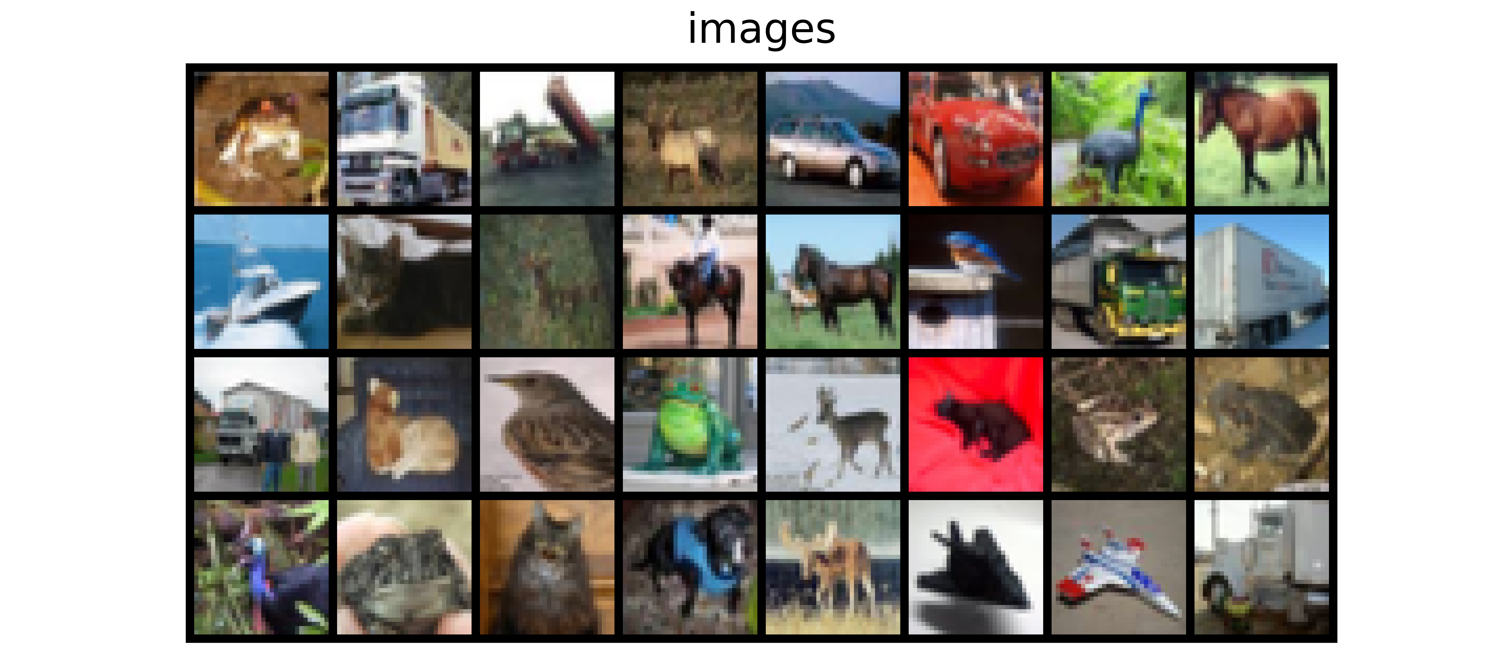

Since we are training an autoencoder which is basically unsupervised, we do not need to class labels meaning we can just extract the images themselves. For visualization sake, we will extract images from each class so as to see how well the autoencoder does in reconstructing images in all classes.

def extract_each_class(dataset):
  """
  This function searches for and returns
  one image per class
  """
  images = []
  ITERATE = True
  i = 0
  j = 0

  while ITERATE:
    for label in tqdm_regular(dataset.targets):
      if label==j:
        images.append(dataset.data[i])
        print(f'class {j} found')
        i+=1
        j+=1
        if j==10:
          ITERATE = False
      else:
        i+=1

  return images
  
  
#  extracting training images
training_images = [x for x in training_set.data]

#  extracting validation images
validation_images = [x for x in validation_set.data]

#  extracting validation images
test_images = extract_each_class(validation_set)

Next, we need to define a PyTorch dataset class so as to be able to use our dataset in training a PyTorch model. This is done in the following code cell.

#  defining dataset class
class CustomCIFAR10(Dataset):
  def __init__(self, data, transforms=None):
    self.data = data
    self.transforms = transforms

  def __len__(self):
    return len(self.data)

  def __getitem__(self, idx):
    image = self.data[idx]

    if self.transforms!=None:
      image = self.transforms(image)
    return image
    
    
#  creating pytorch datasets
training_data = CustomCIFAR10(training_images, transforms=transforms.Compose([transforms.ToTensor(),
                                                                              transforms.Normalize((0.5, 0.5, 0.5), (0.5, 0.5, 0.5))]))
validation_data = CustomCIFAR10(validation_images, transforms=transforms.Compose([transforms.ToTensor(),
                                                                                  transforms.Normalize((0.5, 0.5, 0.5), (0.5, 0.5, 0.5))]))
test_data = CustomCIFAR10(test_images, transforms=transforms.Compose([transforms.ToTensor(),
                                                                                  transforms.Normalize((0.5, 0.5, 0.5), (0.5, 0.5, 0.5))]))

Autoencoder Architecture

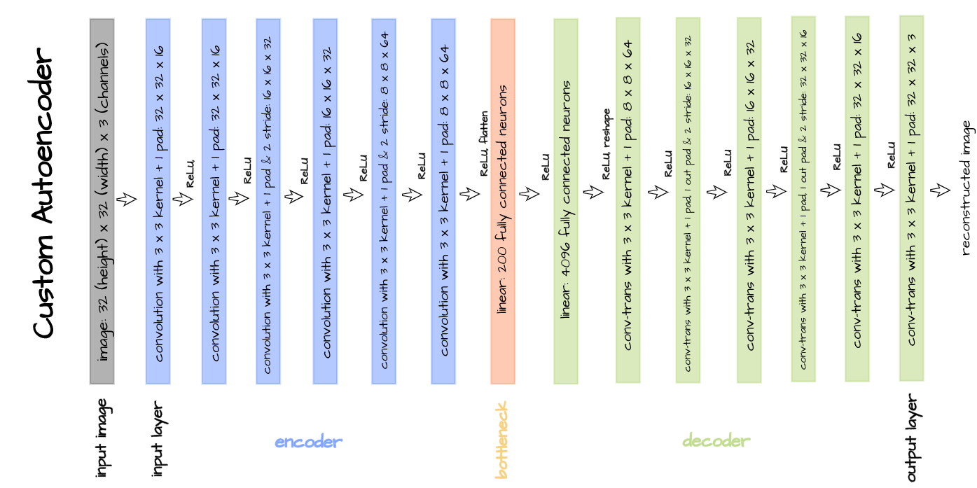
The autoencoder architecture pictured above is implemented in the code block below and will be used for training purposes. This autoencoder is custom built just for illustration purposes and is specifically tailored to the CIFAR-10 dataset. A bottleneck size of 1000 is used for this particular article instead of 200.

#  defining encoder
class Encoder(nn.Module):
  def __init__(self, in_channels=3, out_channels=16, latent_dim=1000, act_fn=nn.ReLU()):
    super().__init__()

    self.net = nn.Sequential(
        nn.Conv2d(in_channels, out_channels, 3, padding=1), # (32, 32)
        act_fn,
        nn.Conv2d(out_channels, out_channels, 3, padding=1), 
        act_fn,
        nn.Conv2d(out_channels, 2*out_channels, 3, padding=1, stride=2), # (16, 16)
        act_fn,
        nn.Conv2d(2*out_channels, 2*out_channels, 3, padding=1),
        act_fn,
        nn.Conv2d(2*out_channels, 4*out_channels, 3, padding=1, stride=2), # (8, 8)
        act_fn,
        nn.Conv2d(4*out_channels, 4*out_channels, 3, padding=1),
        act_fn,
        nn.Flatten(),
        nn.Linear(4*out_channels*8*8, latent_dim),
        act_fn
    )

  def forward(self, x):
    x = x.view(-1, 3, 32, 32)
    output = self.net(x)
    return output


#  defining decoder
class Decoder(nn.Module):
  def __init__(self, in_channels=3, out_channels=16, latent_dim=1000, act_fn=nn.ReLU()):
    super().__init__()

    self.out_channels = out_channels

    self.linear = nn.Sequential(
        nn.Linear(latent_dim, 4*out_channels*8*8),
        act_fn
    )

    self.conv = nn.Sequential(
        nn.ConvTranspose2d(4*out_channels, 4*out_channels, 3, padding=1), # (8, 8)
        act_fn,
        nn.ConvTranspose2d(4*out_channels, 2*out_channels, 3, padding=1, 
                           stride=2, output_padding=1), # (16, 16)
        act_fn,
        nn.ConvTranspose2d(2*out_channels, 2*out_channels, 3, padding=1),
        act_fn,
        nn.ConvTranspose2d(2*out_channels, out_channels, 3, padding=1, 
                           stride=2, output_padding=1), # (32, 32)
        act_fn,
        nn.ConvTranspose2d(out_channels, out_channels, 3, padding=1),
        act_fn,
        nn.ConvTranspose2d(out_channels, in_channels, 3, padding=1)
    )

  def forward(self, x):
    output = self.linear(x)
    output = output.view(-1, 4*self.out_channels, 8, 8)
    output = self.conv(output)
    return output


#  defining autoencoder
class Autoencoder(nn.Module):
  def __init__(self, encoder, decoder):
    super().__init__()
    self.encoder = encoder
    self.encoder.to(device)

    self.decoder = decoder
    self.decoder.to(device)

  def forward(self, x):
    encoded = self.encoder(x)
    decoded = self.decoder(encoded)
    return decoded

Convolutional Autoencoder Class

So as to neatly package model training and utilization into a single object, a convolutional autoencoder class is defined as seen below. This class has utilization methods such as autoencode which facilitates the entire autoencoding process, encode which triggers the encoder and bottleneck returning a 1000 element vector encoding and decode which takes a 1000 element vector as input and attempts to reconstruct an image.

class ConvolutionalAutoencoder():
  def __init__(self, autoencoder):
    self.network = autoencoder
    self.optimizer = torch.optim.Adam(self.network.parameters(), lr=1e-3)

  def train(self, loss_function, epochs, batch_size, 
            training_set, validation_set, test_set):
    
    #  creating log
    log_dict = {
        'training_loss_per_batch': [],
        'validation_loss_per_batch': [],
        'visualizations': []
    } 

    #  defining weight initialization function
    def init_weights(module):
      if isinstance(module, nn.Conv2d):
        torch.nn.init.xavier_uniform_(module.weight)
        module.bias.data.fill_(0.01)
      elif isinstance(module, nn.Linear):
        torch.nn.init.xavier_uniform_(module.weight)
        module.bias.data.fill_(0.01)

    #  initializing network weights
    self.network.apply(init_weights)

    #  creating dataloaders
    train_loader = DataLoader(training_set, batch_size)
    val_loader = DataLoader(validation_set, batch_size)
    test_loader = DataLoader(test_set, 10)

    #  setting convnet to training mode
    self.network.train()
    self.network.to(device)

    for epoch in range(epochs):
      print(f'Epoch {epoch+1}/{epochs}')
      train_losses = []

      #------------
      #  TRAINING
      #------------
      print('training...')
      for images in tqdm(train_loader):
        #  zeroing gradients
        self.optimizer.zero_grad()
        #  sending images to device
        images = images.to(device)
        #  reconstructing images
        output = self.network(images)
        #  computing loss
        loss = loss_function(output, images.view(-1, 3, 32, 32))
        #  calculating gradients
        loss.backward()
        #  optimizing weights
        self.optimizer.step()

        #--------------
        # LOGGING
        #--------------
        log_dict['training_loss_per_batch'].append(loss.item())

      #--------------
      # VALIDATION
      #--------------
      print('validating...')
      for val_images in tqdm(val_loader):
        with torch.no_grad():
          #  sending validation images to device
          val_images = val_images.to(device)
          #  reconstructing images
          output = self.network(val_images)
          #  computing validation loss
          val_loss = loss_function(output, val_images.view(-1, 3, 32, 32))

        #--------------
        # LOGGING
        #--------------
        log_dict['validation_loss_per_batch'].append(val_loss.item())


      #--------------
      # VISUALISATION
      #--------------
      print(f'training_loss: {round(loss.item(), 4)} validation_loss: {round(val_loss.item(), 4)}')

      for test_images in test_loader:
        #  sending test images to device
        test_images = test_images.to(device)
        with torch.no_grad():
          #  reconstructing test images
          reconstructed_imgs = self.network(test_images)
        #  sending reconstructed and images to cpu to allow for visualization
        reconstructed_imgs = reconstructed_imgs.cpu()
        test_images = test_images.cpu()

        #  visualisation
        imgs = torch.stack([test_images.view(-1, 3, 32, 32), reconstructed_imgs], 
                          dim=1).flatten(0,1)
        grid = make_grid(imgs, nrow=10, normalize=True, padding=1)
        grid = grid.permute(1, 2, 0)
        plt.figure(dpi=170)
        plt.title('Original/Reconstructed')
        plt.imshow(grid)
        log_dict['visualizations'].append(grid)
        plt.axis('off')
        plt.show()
      
    return log_dict

  def autoencode(self, x):
    return self.network(x)

  def encode(self, x):
    encoder = self.network.encoder
    return encoder(x)
  
  def decode(self, x):
    decoder = self.network.decoder
    return decoder(x)

With everything setup, the autoencoder can now be trained by instantiating it, and calling the train method with parameters as seen below.

#  training model
model = ConvolutionalAutoencoder(Autoencoder(Encoder(), Decoder()))

log_dict = model.train(nn.MSELoss(), epochs=15, batch_size=64, 
                       training_set=training_data, validation_set=validation_data,
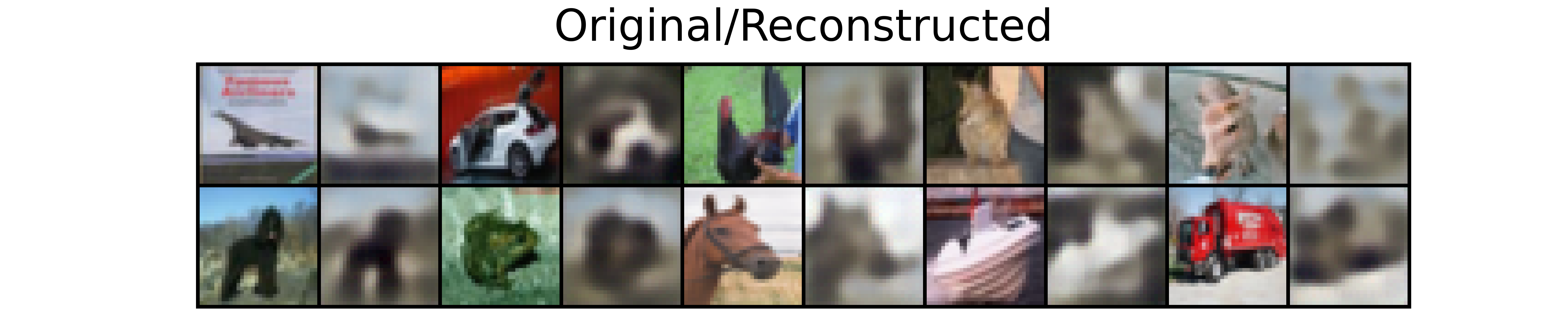
                       test_set=test_data)

After the first epoch, we can see that the autoencoder has began to learn representations strong enough to be able to put together input images albeit without much detail.

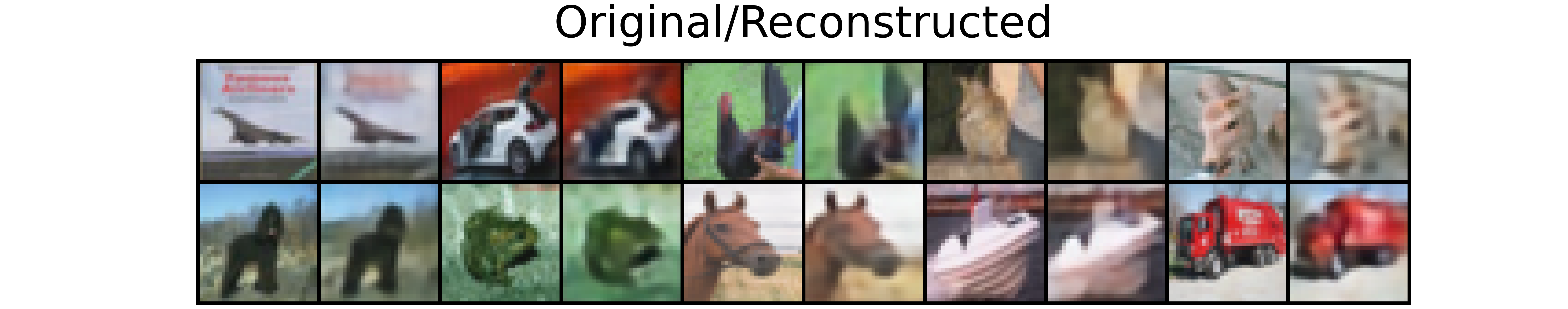
However, by the 15th epoch the autoencoder has began to put together input images in more detail with accurate colors and better form.

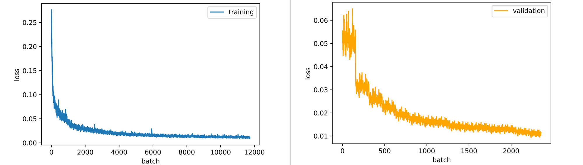
Looking at the training and validation loss plots, both plots are down-trending,  and, therefore, the model will in fact benefit from more epochs of training. However, for this article training for 15 epochs is deemed sufficient enough.

Writing a Visual Similarity Function

Now, that an autoencoder has been trained to reconstruct images of all 10 classes in the CIFAR-10 dataset, we can proceed to use the autoencoder's encoder as a feature extractor for any set of images and then compare extracted features using cosine similarity.

In our case, let's write a function capable of receiving any image as input after which it looks through a set of images (we will be using the validation set for this purpose) for similar images. The function is defined below as described; care must be taken to preprocess the input image just as training images were preprocessed since this is what the model expects.

def visual_similarity(filepath, model, dataset, features):
  """
  This function replicates the visual similarity process
  as defined previously.
  """
  #  reading image
  image = cv2.imread(filepath)
  image = cv2.cvtColor(image, cv2.COLOR_BGR2RGB)
  image = cv2.resize(image, (32, 32))

  #  converting image to tensor/preprocessing image
  my_transforms=transforms.Compose([transforms.ToTensor(),
                                    transforms.Normalize((0.5, 0.5, 0.5), (0.5, 0.5, 0.5))])
  image = my_transforms(image)

  #  encoding image
  image = image.to(device)
  with torch.no_grad():
    image_encoding = model.encode(image)

  #  computing similarity scores
  similarity_scores = [F.cosine_similarity(image_encoding, x) for x in features]
  similarity_scores = [x.cpu().detach().item() for x in similarity_scores]
  similarity_scores = [round(x, 3) for x in similarity_scores]
 
  #  creating pandas series
  scores = pd.Series(similarity_scores)
  scores = scores.sort_values(ascending=False)

  #  deriving the most similar image
  idx = scores.index[0]
  most_similar = [image, dataset[idx]]

  #  visualization
  grid = make_grid(most_similar, normalize=True, padding=1)
  grid = grid.permute(1,2,0)
  plt.figure(dpi=100)
  plt.title('uploaded/most_similar')
  plt.axis('off')
  plt.imshow(grid)

  print(f'similarity score = {scores[idx]}')
  pass

Since we are going to be comparing the uploaded image to images in the validation set we could save time by extracting features from all 1000 images prior to using the function. This process would as well have been written into the similarity function but it will come at the expense of compute time. This is done below.

#  extracting features from images in the validation set
with torch.no_grad():
  image_features = [model.encode(x.to(device)) for x in tqdm_regular(validation_data)]

Computing Similarity

In this section, some images will be supplied to the visual similarity function in a bid to access the results produced. It should be borne in mind however that only images in classes present in the training set will produce reasonable results.  

Image 1

Consider the image of a German Shepard with a white background as seen below. This dog is has a predominantly golden coat with a black saddle and it is observed to be standing at alert facing the left.  

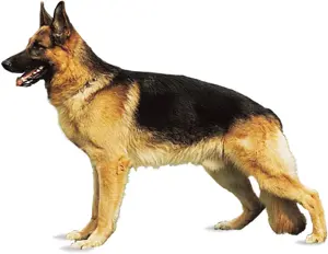
Upon passing this image to the visual similarity function, a plot of the uploaded image against the most similar image in the validation set is produced. Note that the original image was downsized to 32 x 32 pixels as required by the model.

visual_similarity('image_1.jpg', model=model, 
                  dataset=validation_data, 
                  features=image_features)

From the result, a white background image of a seemingly dark coat dog standing at alert facing the left is returned with a similarity score of 92.2%. In this case, the model essentially finds an image which matches most of the details of the original which is exactly what we want.

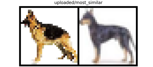
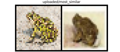
Image 2

The image below is that of a generally brownish looking frog in a prone position facing the rightward direction on a white background. Again, passing the image through our visual similarity function produces a plot of the uploaded image against it's most similar image.

visual_similarity('image_2.jpg', model=model, 
                  dataset=validation_data, 
                  features=image_features)

From the resulting plot, a somewhat gray looking frog in a similar position (prone) to our uploaded image is returned with a similarity score of about 91%. Notice that the image is also depicted on a white background.

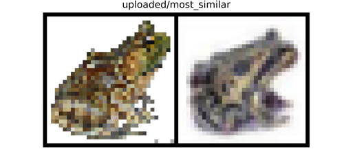
Image 3

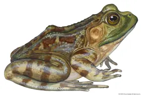
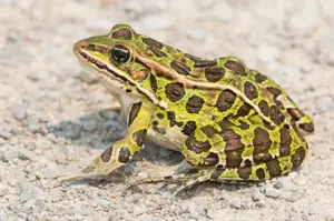
Lastly, below we have an image of another frog. This frog is of greenish coloration in a similarly prone position to the frog in the previous image but with distinctions of facing the leftward direction and being depicted on a textured background (sand in this case).

visual_similarity('image_3.jpg', model=model, 
                  dataset=validation_data, 
                  features=image_features)

Just like in the previous two sections, when the image is supplied to the visual similarity function a plot of the original image and the most similar image found in the validation set is returned. The most similar image in this case is that of a brownish looking frog in a prone position, facing the leftward direction, depicted on a textured background as well. A similarity score of approximately 90% is returned.

From the images used as examples in this section it can be seen that the visual similarity function works as it should. However, with more epochs of training or perhaps a better architecture, there is a possibility that better similarity recommendations will be made beyond the first few most similar images.

Final Remarks

In this article, we were able to look at another beneficial use of autoencoders, this time as a tool for visual similarity recommendation. Here we explored how an autoencoder's encoder can be used as a feature extractor with the extracted features then compared using cosine similarity in order to find similar images.

Basically all the autoencoder does in this instance is to extract features. Indeed, if you are quite conversant with convolutional neural networks, then you will agree that not only autoencoders could serve as feature extractors, but that networks used for classification purposes could also be used for feature extraction. Thus, this implies their utility for visual similarity tasks in turn.