As data scientists, machine learning engineers, and ML/deep learning hobbyists, many of us have had the experience of trying to choose the optimal platform for conducting cloud computing. Getting more compute is often necessary, especially now while the current problems in the shipping industry are sharply raising already high prices on GPU's. Furthermore, even if availability isn't a problem, it is not always cost effective to purchase a GPU. Often, it is optimal to use a ML ops platform to get the most cost effective access to your computing needs.

Every platform has a variety of different available GPU and CPU types for their remote machines, and there is some degree of variation between competitors as well over which they carry. These can range from older, weaker, GPU like a Maxwell generation to cutting edge GPU's like those from the Ampere series. These very greatly in terms of capabilities, and each come attached with a number of helpful specs like GPU memory on every website. For many of us, this is sufficient for choosing a machine. For many others, this can be where problems begin to be encountered. How do we select the best GPU for our needs?

When choosing a GPU from Paperspace, for either Core or Gradient, it can be challenging for those without domain knowledge to know what GPU to select. While it may be obvious that more GPU memory and a higher price will likely indicate a better machine, choosing a GPU that isn't the cheapest or the most expensive is something many would just avoid considering. This isn't cost effective, but it can be challenging to dive into the hardware world and really understand the differences between the options.

In the interest of helping this process, this blog post will breakdown the power and cost differences between the available GPU machines in the context of a series of three computer vision related deep learning benchmarks. We'll consider these benchmarks in two contexts: time to completion and max batch size. We will then propose a series of recommendations based on speed, power, and cost.

Terms to know

• Throughput/Bandwidth: a measure of how many times a task can be completed within a set period. Measured in Gigabytes per second.
• GPU Memory: The available memory that the GPU can use to process the data, in Gigabytes.
• Time to solution: the amount of time that is measured for the task to be completed. This can be training time, generation time, etc, and will be measured in seconds.
• Maximum batch input size: the maximum size of each batch that can be processed by the NN/model before risking running out of memory.

Paperspace Machine Facts:

*note: the M4000 is actually always free on Gradient. We are using the Core pricing. This is for the sake of comparison. The P5000 and RTX5000 also have free options with the Pro plan.

Let's take a look at the relevant data we already know for Paperspace GPUs. Included in the table above in particular are the GPU memory, memory bandwidth, and price per month values. These are going to be what we use to help calculate our benchmark comparisons in terms of cost. You should always select your GPU based on these factors, as they translate indirectly to power, speed, and the cost efficiency of running the model for a full month, 24 hours per day or for a total of 720 hours.

We've included a heat map running along each of the bottom 4 rows. The green cells indicate the more cost effective options based on these metrics, and the red indicates the more expensive options. Let's look at our GPU options in this context first.

While the A100 is pricier than about half the alternatives in terms of efficiency, it's always tempting to default to the top option in terms of GPU memory. This can be overkill in terms of compute power, and the cost is high (though cheaper than other options like AWS), but it will always be the fastest thanks to its massive throughput. Others may default to the free M4000, taking advantage of the free Notebook type all users on Gradient have access to. But if you are running production ML, you will always be losing out on potential efficiency by choosing to use the M4000. Other paid options can accomplish the same task much more quickly, and that is often worth the payment. Based on looking at these extremes of the options, choosing the most expensive or cheap option is always tempting, but it's not efficient.

Instead, this benchmark and GPU spec guide was created to help you choose the best option for your task on Gradient. For example, instead of an M4000, consider using the RTX4000 machine. Upgrading to the Growth plan will make the RTX4000 completely free to use for just 8 dollars per month, and is effectively a one to one upgrade for all tasks at a relatively low cost. If you need more power, the Ampere series GPUs such as the A4000, A5000, and A6000 will likely be the most cost efficient options.

We want anyone reading this to be able to better discern what their needs are, and then guide them towards the appropriate machine type for their task. With these thoughts in mind, let's look at the benchmarks, and see each machine type performs in practice compared to one another.

Assumptions and notes for benchmarking:

Below are a list of assumptions and notes we made while doing the benchmarking, as well as a few for you to keep in mind. Consider each one and how this may have affected our interpretation of the outcomes in order to get a full understanding of the benchmark reasoning.

• The model benchmarks will achieve a satisfactory enough quality in their completion of the tasks to not merit reporting any sort of evaluation metric. Model efficacy is irrelevant to measuring the training time because each GPU will still each undergo the same tasks, and it is irrelevant to the inference time because the pre-trained YOLOR model we will use has already been evaluated to be effective. Furthermore, one of the benchmarks has a purposefully lowered number of epochs to the point of uselessness in any other practice.
• All other tasks (other notebook kernels) will be cleared from the console, so that no additional memory is being taken up by other processes.
• The data we are using is optimized for this task. Less optimal datasets may introduce different effects to chronological aspects of a deep learning model's training and inference.
• The M4000 can only be accessed for free on Gradient. We are using an approximate sample price based on the Paperspace Core pricing.
• All A4000, A5000, and A6000 instances have 48.3 GB of CPU memory, and all A100 instances have 96.6 GB of CPU memory. All other instances have 32.2 GB of CPU memory.  
• In GPU names, the letter out front represents the GPU generation. These are namely Maxwell, Pascal, Volta, Turing, and Ampere, ordered by how recently they were introduced.  Generally speaking, newer architectures with similar specs to older ones will outperform the older ones.
• All benchmarks were completed on Paperspace Gradient.

Benchmark tasks:

Object recognition detection - YOLOR-CSP-X on video

YOLOR or "You only learn one representation" is a new algorithm for object detection and recognition. We are using it today to generate predictions of the objects held in a youtube video. Since object recognition and detection are computationally heavy tasks, these will show us directly how quickly each GPU is able to use the model to make the predictions, and from that we can make comparative inferences about their performance.

Inference parameters:

cfg cfg/yolor_csp_x.cfg #config file
weights yolor_csp_x.pt 
conf-thres 0.25 # object confidence threshold
img-size 1280 # img size to load in frames as
device 0 # our GPU

Image Classification - EfficientNet with tiny-image-net200

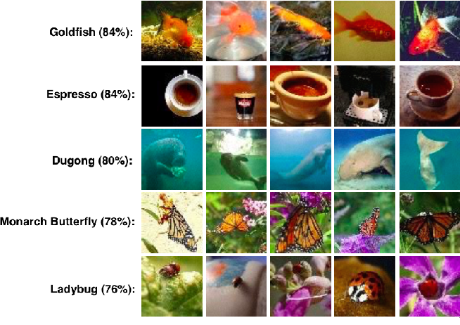
For our next example, we will take on one of the most common use cases for deep learning: image classification. We are going to implement EfficientNet on the tiny-imagenet-200 dataset (which can be freely mounted from public datasets onto any Notebook), and use the varying times it takes to train the classifier as our measurement of efficiency as well as the maximum batch size it can intake. This will serve as our more conventional example for a deep learning model.

This test is based on this tutorial on image classification.

Training parameters:

batch_size = 256
lr = 0.001  # Learning rate
num_epochs = 1  # Number of epochs
log_interval = 300  # Number of iterations before logging
loss_func = nn.CrossEntropyLoss()
optimizer = optim.Adam(model.parameters(), lr=lr)

Image Generation - StyleGAN_XL image generation

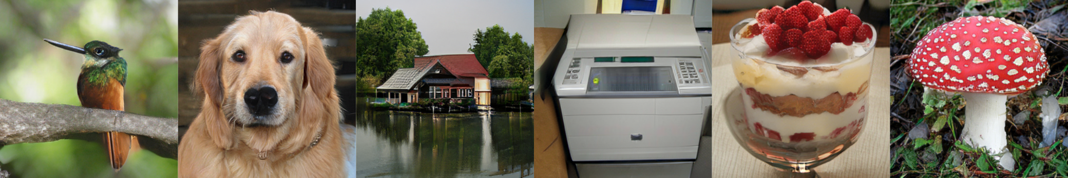
Finally, we will use StyleGAN_XL, a recently released implementation of the StyleGAN framework aimed at generating 1024 x 1024 resolution images, to benchmark image synthesis model training times. Since image synthesis is so costly, we included this to serve as a good example of how the different GPUs perform on computationally heavy tasks. Furthermore, this task will differ from the image classification task further by working with expensive high quality images for training.

Training parameters:

cfg=stylegan3-t #StyleGAN config
data=stylegan_xl/data/pokemon256.zip
gpus=1 #number of GPUs
batch=8 #batch size 
kimg 5 # size of subset to process in each epoch
metrics none

Benchmark Results:

Throughput:

Best GPU: Throughput

Best GPU in terms of throughput: A100. Use this GPU when you need to quickly process a significant amount of data.

Best GPU pricing per GB/minute: RTX4000. Use this GPU when you need to quickly process big data on a budget.

Best GPU for budgeting: RTX4000. Use this GPU when saving on cost is the primary goal

Justification:

Before jumping into the benchmark tasks, let's focus for a second on one of the measurements listed above: throughput. Throughput, or bandwidth, is very useful for getting an idea for the speed at which our GPUs perform their tasks. It is literally a measurement of the amount of GB/s that can be processed, and can be effectively considered the measurement of its processing speed. This measure differs from the overall memory capacity of the machine because certain architectures are more capable than others at making use of their increased capacity.

This effectively works to make these options cheaper, like how using the RTX5000's capabilities are less affordable when compared to those of the similar A4000 on the basis of throughput.  You can use throughput to estimate the cost efficiency of the different GPUs as a function of the relationship between time and the cost to lease the machine.  Using this information, we can better consider weaker GPU options from the same generation that get comparable performance on throughput. This is especially good to consider when cost over time is more important than speed, like with the RTX4000 and the A5000. That being said, the A100 actually compares well in terms of cost efficiency for throughput.

Looking at throughput gave us an abstract idea for how to compare the different GPU offerings, let's now look at the computer vision benchmarks to see how the different values listed in the tables above actually affect a model's time to completion for examples in training and inference.

Time to completion:

*OOM: Out of Memory. This indicates the training failed due to lacking memory resources in the kernel.

** Single run cost: Time in seconds was converted to hours, and then multiplied by the cost per hour. Reflects the cost of a single run of the task on the GPU.

Time to completion is a measure, in seconds, of the time it takes for the model to train or, in the case of YOLOR, make an inference. We chose this metric for our benchmark because it is intuitively useful for understanding the differences in capability between the different GPU offerings. For example, it can give us insight for how different values like GPU memory and throughput affect the different model's training times. We used 3 - 5 recorded wall times for each task to get the average wall times reported above. The first recorded value was not included, as various downloading tasks or set up tasks that needed to run were causing these entries to be significantly slower than following runs.

Best GPU: Time to completion

Best GPU in terms of time to completion: A100. Use the A1000 when you want to complete your task as quickly as possible.

Best GPU as a function of cost to run: A4000. Use the A4000 to complete tasks quickly while saving on cost.

Best GPU for budgeting: RTX5000. Use the RTX5000 when cost is the most important factor.

Justifications:

YOLOR

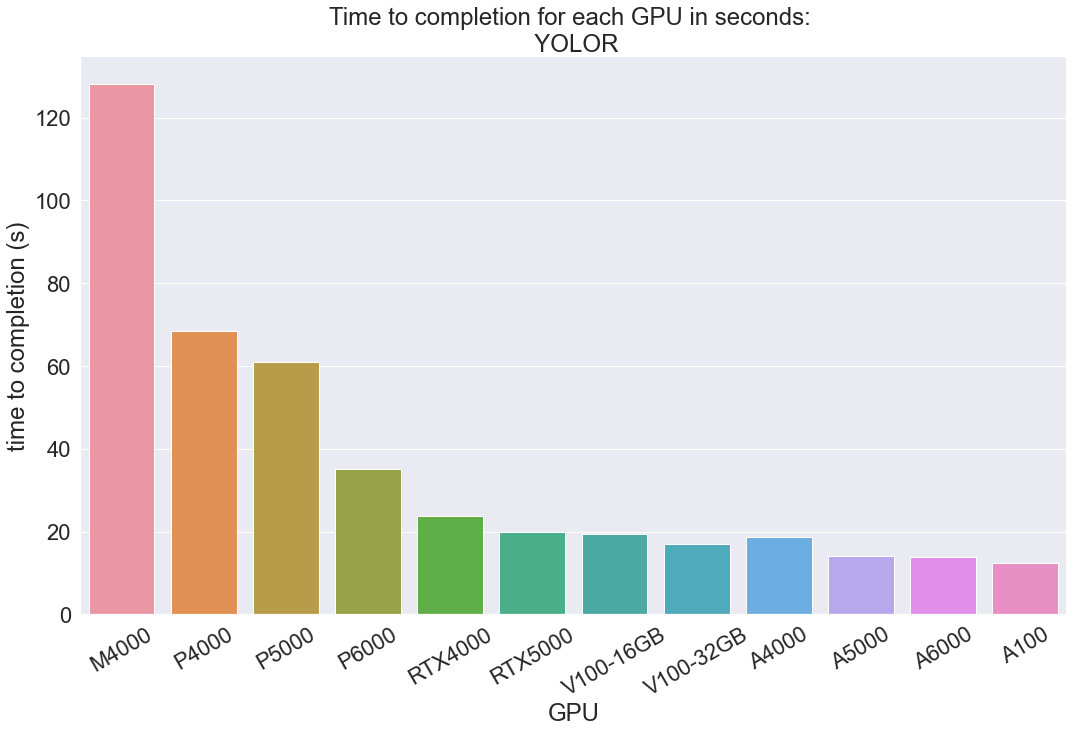
Our quickest task, YOLOR compares the speeds for recognizing objects in a short YouTube video. As you can see, this task has revealed that there are some clear differences between the completion times for each of the different GPU generations. The Maxwell and Pascal GPU architectures are older and less efficient. The low throughput values for these is reflected in their lower time to completion values. For example, while the Turing RTX4000 has the same amount of GPU memory as the Pascal P5000, it is much faster due to its higher throughput and more contemporary architecture. On the other side, the A4000 also has similar GPU RAM, but is faster than the RTX4000 thanks to its newer architecture enabling a higher throughput. Higher GPU memory can overwhelm this effect, however, as shown by the Volta V100's outperforming the newer, but less powerful, RTX5000. Finally, the Ampere series GPUs with the newest architectures, highest throughput values, and RAM performed the inferences the most quickly. The A100 was always the fastest, despite having less RAM than the A6000. This is likely due to the near double throughput present in the A100 compared to the A6000.  

StyleGAN_XL

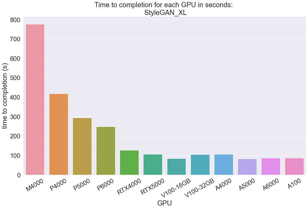
StyleGAN_XL involves training this large, new implementation of the popular StyleGAN framework on a collection of images of Pokemon. Looking at the table above, we can see a similar pattern to the same results we did with the inference task on YOLOR. The Maxwell and Pascal were again the far slower options, then the Turing RTX GPUs, the V100s, and fastest were the Ampere series.

There were a few outliers here that don't seem to be reflected in the GPU specs. Across multiple Notebooks, the A5000 outperformed the A6000 and A100, and the V100 16GB outperformed the V100 32GB. This is likely just a quirk of this particular training task, so we don't take too much stock in the incredible performance of the V100 16GB and A5000 here. You will likely still find better value in the V100 32GB and A100, respectively. Despite these outliers, these findings further indicate that the A100 and other Ampere series GPUs are extremely fast. The next best options in the Volta GPUs are far more expensive, so selecting an A5000 or A6000 on this task seems to be the most cost effective.

EfficientNet

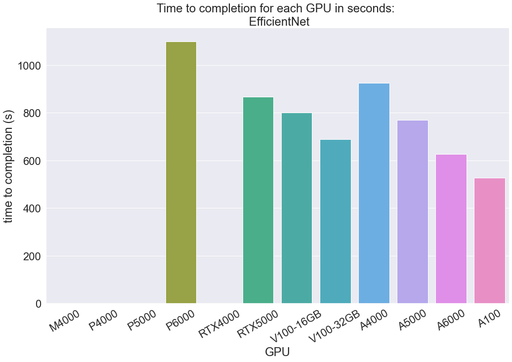
The EfficientNet classification task was where we wanted to push the GPUs in terms of input size. We chose to use a relatively large batch size of 64 across all the tests here in order to see how quickly each GPU can process these relatively large input batch sizes. While the tiny-imagenet-200 images are relatively low resolution, 64 x 64, they are still RGB images and expensive to process. As you can see, this took much longer than the other two tasks, and some of the GPUs ran out of memory before completion (M4000, P4000, P5000, and RTX4000). This was expected, as we wanted to provide an example where we stretch the capabilities of these GPUs to their limits and show how some Pascal and Maxwell instances may not be up to your task.

This task displayed the same pattern of training times as shown by the YOLOR task. The Pascal and Maxwell generation machines struggled to complete the task at all, and the P6000 was comparatively the slowest in doing so, despite running. The RTX5000 on the other hand continued its trend of being very cost effective. While slower than the tests run on other machines, the cost makes this a very attractive option when time is not a major expense factor. The Volta and Ampere series GPUs performed the fastest by far, and the outliers in the previous benchmark, the V100s and A5000, returned to expected behavior in this task.

Maximum Batch Input Size (batch size: int):

Testing the maximum batch size for the input provides us with an idea of how much data the model is capable of processing at each update stage for each GPU. In our cases, the max batch size tells us how many images the models can process per iteration before running out of memory. Therefore, the maximum batch input size is an indirect measure of how expensive a task can be before the GPU can no longer handle it.

Best GPU: Max batch size

Best GPU at handling large batch sizes: A6000. This GPU actually has more memory and CUDA cores than the A100, but a lower throughput. If we need to handle a more expensive task, then the A6000 is the best option.

Best GPU in terms of cost per batch item: A6000. The A6000 is also the most cost effective for both training tasks. In terms of per item processing, the A6000 has the best ratio of cost to item processed. The P6000 is also a fantastic option.

Best GPU for budgeting: A4000. The overall cost per hour and cost per batch item are comparatively low for both tasks on an A4000. The A4000 performed nearly as well as the A6000 at under half the price point, and the StyleGAN_XL performance indicates it may do better than the A6000 in terms of cost efficiency.  

Justifications:

StyleGAN_XL:

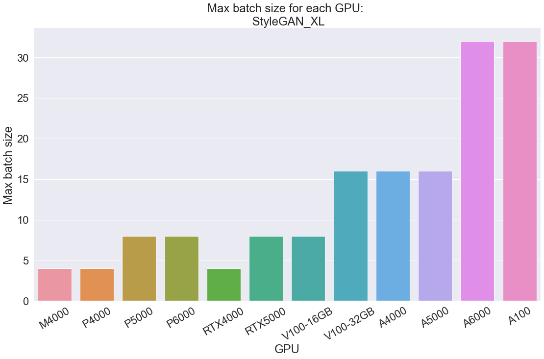
The StyleGAN_XL task is specifically aimed at training a model to generate high quality, 1024 x 1024 resolution images. As a result, the images we are inputting are quite a bit higher quality (1280x1280) than than those of tiny-imagenet-200 (64 x 64) and require more GPU power to process. This is why the batch sizes are so much smaller than in the EfficientNet tests.

Unsurprisingly,  a similar pattern appears above as we saw on the time to completion tests. As we go up in generation and GPU memory, these values rise in tandem. With only 8 GB of RAM, this is why the M4000, P4000, and RTX4000 can only manage a batch size of 4. The larger memory Pascal and RTX GPUs perform a bit better, but the large memory of the Volta and Ampere GPUs often leave them low performant by comparison. On the other hand, the A6000 and A100 have memories of 48 and 40 GB respectively. This allows them to handle the largest batch size we could collect for this task, 32.

In terms of cost, the Ampere series GPUs are clear standouts in cost per batch item processed. This is likely a direct result of the cross section of high GPU memory, throughput, and CUDA cores in each of these GPU types. The A6000 and A4000 appear to be the most cost effective overall, at 5 - 6 cents per item. The V100 16 GB ends up being revealed as the least cost efficient by this metric, likely due to the older Volta architecture not being as proficient as the RTX or Ampere GPUs for processing large batches of data while having the second highest run cost at $2.30 per hour.  

EfficientNet

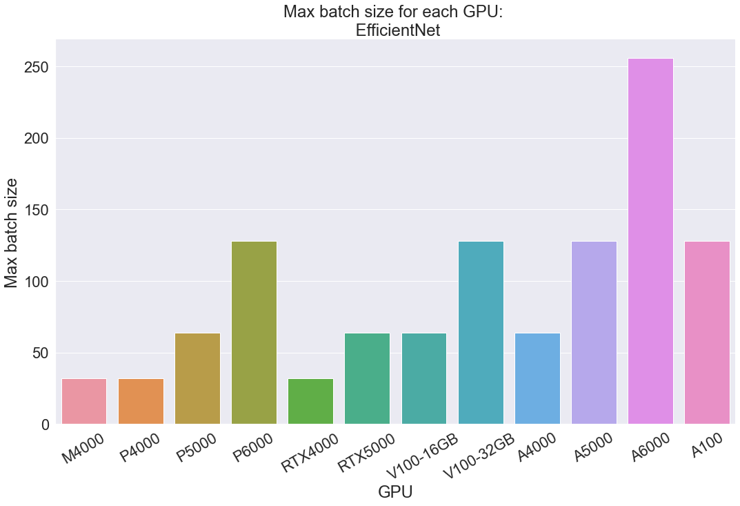
The EfficientNet test with tiny-imagenet-200 is great for showing batch size because even the weaker GPUs can process a decent amount of 64 x 64 images without any issue. We can use the test to get a better intuitive understanding of the magnitude of difference between the batch sizes across the different testing conditions.

With EfficientNet, the same 3 instances we saw struggling with StyleGAN XL again reflected their relative weakness. The M4000, P4000, and RTX4000 each, with only 8 GB of memory, struggle to handle more than 32 images at this much lower resolution. After them, a new pattern emerges based on GPU memory. The more powerful Pascal P5000 and P6000 get 64 and 128 respectively, showing a clear jump with each boost in RAM. Similarly, the RTX5000 GPU can work with up to a batch size of 64. The A6000 performed the best with 256, and the P6000, 32 GB V100, A5000, and A100 tied for second with 128. Scrolling back up to our facts table, we can see that these GPUs have 24, 32, 24 and 40 GB of memory each. This likely means that processing a batch size of 256 becomes possible with somewhere between 40 and 48 GB of memory. From all of this, we can clearly infer a direct relationship between the max batch size and the GPU memory.

As for cost, the V100 16 GB is notably inefficient again. As it did with StyleGAN_XL, it has the second lowest possible batch size paired with a high cost per hour that gives some unattractive rates in comparison to the other options.

The second worst option is the A100, which has the highest cost per hour. We didn't want to remove this data, but this is likely misleading. The A100 is still the second most effective at handling large batch sizes in this task. After it, the RTX5000, V100 32GB, M4000, P4000, and P5000 seem to represent around the average in terms of cost per item.

The best options for running EfficientNet, based on the ratio of cost to batch size, are the three remaining Ampere GPUs and the P6000. The A4000 and A5000 perform well and only cost just over a cent per item processed, but the P6000 and A6000 break below the one cent range. This is a direct reflection of the comparatively high amount of memory in each instance (24 GB and 48 GB respectively) paired with the relatively low cost to run them. The P6000 has the same memory size as the A5000, but is about 80% as expensive to run. Meanwhile, the A6000 is about 60% as expensive as the A100, and can handle a larger batch size at nearly the same speed. Based on this information, if you need to use a large batch size, in terms of the items file size or the size of the batch itself, consider using the A6000 or the A5000.

Concluding arguments

Based on the benchmarks and specs we examined above, we can now try to form a full conclusion for what GPUs perform best on Paperspace Gradient for different tasks. This was done through a series of inference and training tasks using YOLOR, StyleGAN_XL, and EfficientNet. Using measurements of time and batch size, along with existing information about cost and the GPU specs, we were able to show our recommendations for which GPUs to select based on terms of power, cost, speed, and efficiency.

We will now recommend the best overall GPUs for 4 different situations: when code needs to run fast as possible, when as large an input as possible needs to be processed, and when we want to run the task as inexpensively as possible. These varied situations should cover a wide variety of potential situations our users may run into. While each of these conclusions are based on our benchmarks, they are also reflected in the cost and GPU specs data.

Best GPU: Overall recommendations

When we want to run a model as quickly as possible, regardless of the cost, then the A100 is our recommendation. With the highest throughput at 1555 GB/s, the A100 is the pinnacle of GPU technology that is available to your average consumer, and will always complete the work quickly enough that it's high price will not be a problem. It also has the second highest GPU memory available, 40 GB, so it can take on nearly any task designed for a single GPU. This is without a doubt the best single GPU available on Paperspace in terms of overall performance.

When we want to prepare for the maximum input size possible for a model's training, then the A6000 is our recommendation. With 48 GB of GPU RAM, the A6000 can take on huge batch sizes. This is a reflection of its large volume of GPU memory and solid throughput capacity, and we should always select the A6000 when we need to use a large batch size for training, when we need to access a large amount of other variables, data, or models with the GPU memory, or have a particularly complex task at hand, like image generation. The A6000 is even situationally more appropriate to use than an A100, regardless of the difference in cost!

When we want to run our machine or deep learning code as cheaply as possible, then our recommendation is the A4000. The A4000 is across the board the most efficient option for a GPU in terms of cost efficiency. It has one of the best ratios of throughput to price, time to completion to price, and cost per batch item, and it is still extremely robust at dealing with large amounts of data thanks to its 16 GB of memory.

Note: there are some quirks to setting up the benchmarks that make it difficult to share a Notebook containing the examples. The author is working on making a presentable version, but you can access the Gradient Notebook here.