Constructing Neural Networks From Scratch: Part 1

With the presence of popular deep learning frameworks such as TensorFlow, Keras, PyTorch, and other similar libraries, it has become much easier for a novice in the field to pick up the subject of neural networks at a faster pace. Although these frameworks provide you a path to solving the most complex computations within a few minutes, they don't require you to understand the true core concepts and intuition behind all the requirements. If you have the knowledge of how a specific function works, and how exactly you can make use of that function within your code block, you will solve most problems without too much difficulty. However, for anyone to truly appreciate the concept of neural networks and understand the complete working procedure, it becomes essential to learn how these artificial neural networks work from scratch. How can these neural networks solve these complex problems?

Understanding how neural networks work and, subsequently, how they are constructed is a worthwhile endeavor for anybody interested in AI and deep learning. While we are restricting ourselves from using any kind of deep learning frameworks such as TensorFlow, Keras, or PyTorch, we will still make use of other useful libraries like NumPy for numerical matrix computations. With NumPy arrays, we can perform numerous complex computations that will mimic the effect of deep learning, and use that to build understanding of the procedural workflow of these neural networks. We will implement some neural networks designed to solve a fairly simplistic task with the help of these neural nets built from scratch.

Introduction:

The topic of neural networks is one of the most intriguing within the domain of deep learning and the future of Artificial Intelligence. While the term artificial neural networks is only loosely inspired by the concept of biological neurons, there are a few noticeable similarities that to keep in mind when conceptualizing them. Much like with human neurons, one interesting aspect of using artificial neural networks is that we typically can determine what they are doing, but there is often no explicit way to determine how they work to achieve the goal. While we can potentially answer some of the 'what' aspects, there are numerous discoveries to be made to fully understand everything we need to know about how the model is behaving. This is known as the 'black box' metaphor for deep learning, and it can be applied to a number of deep learning systems. That being said, many neural networks are interpretable enough that we can easily explain their purpose and methodology, and this is dependent on your use case.

Artificial Intelligence is a humungous field in which deep learning and neural networks are just two of the subdomains. In this article, our primary objective is to dive more deeply into the concept of neural networks, and we will proceed to show how to construct an architecture from scratch without making use of some of the prominent and popular deep learning frameworks. Before we dwell on the implementation of the neural network from scratch, let us gain an intuitive understanding of their working procedure.

Understanding the concept of neurons:

Most mathematical operations can be linked through a function. A function is one of the most essential concepts through which a neural network can learn almost anything. Regardless of what the function does, a neural network can be created to approximate that function. This is known as the the Universal Approximation Theorem, and its this law that allows neural networks to work on such a huge variety of different challenges while also giving them their black box nature.

Most real-world problems such as computer vision tasks and natural language processing tasks can also be associated with each other in the form of functions. For example, through functions, we can link the input of a few words to a particular output word and a bunch of images to their respective output image. Most concepts in math and real-world problems can be reframed as a function to frame a problem for which the desired neural network can find the appropriate solution.

What is an Artificial Neural Network and how does it work?

The term Artificial Neural Networks is now commonly referred to as Neural Networks, Neural Nets or nns. These neural nets are loosely inspired on biological neurons. It is important to again note that there is actually very little correlation between the neurons in living entities and the ones used to construct neural network architectures. Although the underlying working procedures of both these elements are quite different, they do share the trait that when these neural networks are combined together, they can solve complex tasks with relative ease.

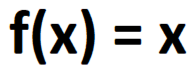
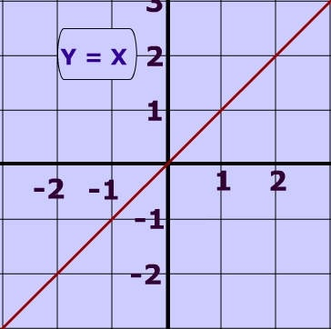
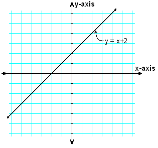
To understand the basic concept of how neural networks work, one of the critical mathematical concepts that we can use to help understand neural networks is the line equation, which is "y = mx + c." The "y = mx" part of the equation helps to manipulate the line to achieve the desired shape and values. The other value, the intercept 'c', helps to vary the positioning of the line by displacing it's intercept on the y axis. Refer to both the images to gain a more clear understanding of this basic concept.

In terms of neural networks, Y = WX +B can be used to represent this equation. Y would represent the output values, 'w' represents the weights that need to be adjusted, 'x' represents the input values, and 'b' represents the values. By using this simple logic, neural networks can use the known information 'b' and 'w' to determine the value for 'x'.

To understand this particular concept of weights and biases better, let us explore a simple code snippet as shown below and the resulting output. Using some input values, weights, and biases, we can compute an output with the dot product of the inputs with the transpose of the weights. To this resulting value, the respective biases are added to compute the desired values. The example below is quite simple, but sufficient for creating a basic understanding. However, we will cover more complex concepts in the next section and in upcoming articles.

import numpy as np

inputs = [1, 2, 3, 2.5]

weights = [[ 0.2, 0.8, - 0.5, 1 ],
           [ 0.5, - 0.91, 0.26, - 0.5 ],
           [ - 0.26, - 0.27, 0.17, 0.87 ]]

biases = [2, 3, 0.5]

outputs = np.dot(weights, inputs) + biases

# Or Use this method 
# np.dot(inputs, weights.T) + biases

print (outputs)

[4.8   1.21  2.385]

When neural networks are collectively combined together, they are able to learn through a training process with the help of backpropagation. The first step is the forward propagation that occurs by computing the necessary information at each layer until the output cell by using random weights. However, these random weights are usually never close to perfect, and the weights need to be adjusted to achieve a more desired result. Hence, backpropagation in neural networks is one of the more crucial aspects of its functionality. Backpropogation is where the weights are manipulated and adjusted, usually with the comparison of the output in hand and the expected output. We will look into these concepts further in the next section and upcoming articles.

Construction of neural networks from scratch:

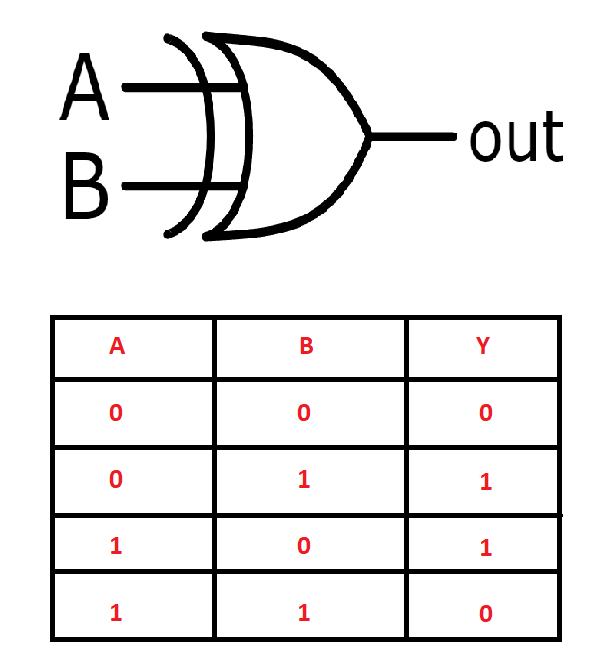
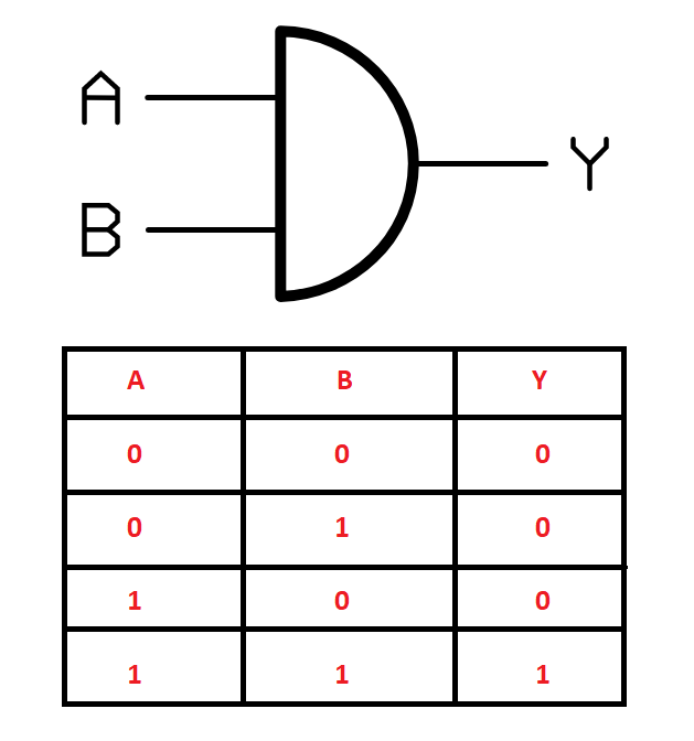
In this section, we will see how to solve some tasks with the help of the construction of neural networks from scratch. Before we start building our neural networks from scratch, let us gain an understanding of the type of problem that we are trying to solve in this article. Our objective is to construct neural networks that can understand and solve the functioning of logic gates, such as AND, OR, NOT, XOR, and other similar logic gates. For this specific example, we will look at how to solve the XOR gate problem by constructing our neural networks from scratch.

Logic gates are some of the most elementary building blocks of electronic components. We are using these logic gates because, as their name suggests, each of these gates operates on a specific logic. For example, the XOR gate only provides a high output when both the input values are different. If both the input values are similar, the resulting output is low. These representations of logic are often represented in the form of a truth table. The image above shows the symbolic and truth table representation of the XOR gate. We can use the input and output values in the form of arrays to train our constructed neural network to achieve desirable results.

Let us first import the necessary libraries that we will utilize for constructing neural networks from scratch. We will not use any deep learning frameworks in this section. We will only use the NumPy library to simplify some of the complex tensor computations and the overall mathematical calculations. You can choose to build neural networks even without the NumPy library, but it would be more time-consuming. We will also import the only other library we need for this section in matplotlib. We will use this library to visualize and plot the loss as we train our model for a specific number of epochs.

import numpy as np
import matplotlib.pyplot as plt

Let us describe the inputs of the truth table and the expected output for the XOR gate. The readers can choose to work on different gates and experiment accordingly (Note that sometimes you not might get the desired results). Below is the code snippet for the input variables and expected outcome for the XOR gate.

a = np.array([0, 0, 1, 1])
b = np.array([0, 1, 0, 1])

# y_and = np.array([[0, 0, 0, 1]])
y_xor = np.array([[0,1,1,0]])

Let us combine the inputs together into a single array entity so that we have one total input array and one output array for the neural network to learn. This combining process can be done in a couple of ways. In the below code block, we are using a list to combine the two arrays and then converting the final list back into the numpy array format. In the next section, I have also mentioned another method of combing this input data.

total_input = []

total_input = [a, b]
    
total_input = np.array(total_input)

The resulting input array is as follows.

array([[0, 0, 1, 1],
       [0, 1, 0, 1]])

For most problems with neural networks, the shape of the arrays is the most critical concept. Shape mismatches are the most likely errors that occur when solving such tasks. Hence, let us print and analyze the shape of the input array.

(2, 4)

Let us now define some of the essential parameters that we will require for constructing our neural network from scratch. The activation function of a node defines the output of that node given an input or set of inputs. We will define the sigmoid function first, which will be our primary activation function for this task. Then, we will proceed to define some of the basic parameters, such as the number of input neurons, hidden neurons, output neurons, the total training samples, and the learning rate at which we will train our neural network.

# Define the sigmoid activation function:
def sigmoid (x):
    return 1/(1 + np.exp(-x))

# Define the number of neurons
input_neurons, hidden_neurons, output_neurons = 2, 2, 1

# Total training examples
samples = total_input.shape[1]

# Learning rate
lr = 0.1

# Define random seed to replicate the outputs
np.random.seed(42)

In the next step, we will initialize the weights that will be passed through the hidden layer and the output layer, as shown in the below code snippet. It is often a good idea to randomize the weights rather than assign them values of zero, as the neural network may sometimes fail to learn the desired outcome.

# Initializing the weights for hidden and output layers

w1 = np.random.rand(hidden_neurons, input_neurons)
w2 = np.random.rand(output_neurons, hidden_neurons)

In the next code block, we will define the working structure of our neural network model. Firstly, we will make the function to perform the forward propagation through the neural network structure. We will start by computing the weights and the input values in the hidden layers, and then passing them through our sigmoid activation function. We will then perform a similar propagation for the output layer as well, where we will utilize the second weights that we previously defined. The randomly generated weights obviously cannot achieve the desired results and need to be fine-tuned. Hence, we will also implement the backpropagation mechanism to help our model train more effectively. This action is performed similarly to how we discussed in the previous section.

# Forward propagation
def forward_prop(w1, w2, x):
    z1 = np.dot(w1, x)
    a1 = sigmoid(z1)    
    z2 = np.dot(w2, a1)
    a2 = sigmoid(z2)
    return z1, a1, z2, a2

# Backward propagation
def back_prop(m, w1, w2, z1, a1, z2, a2, y):
    
    dz2 = a2-y
    dw2 = np.dot(dz2, a1.T)/m
    dz1 = np.dot(w2.T, dz2) * a1*(1-a1)
    dw1 = np.dot(dz1, total_input.T)/m
    dw1 = np.reshape(dw1, w1.shape)
    
    dw2 = np.reshape(dw2,w2.shape)    
    return dz2,dw2,dz1,dw1

Now that we have defined both the forward propagation and backward propagation mechanism, we can proceed to train the neural network. Lets make a training loop to run for a predefined number of iterations. First, we will utilize the forward propagation to receive the output values and then start computing the loss accordingly by comparing it with the expected output. Once we start performing the backpropagation of the neural network, we can start to fine-tune the weights to receive the final result equivalent to the expected outcome. Below is the code block for the training procedure. We are also ensuring that the loss is constantly decreasing, and the neural network is learning how to predict the desired results along with the graph for the following.

losses = []
iterations = 10000

for i in range(iterations):
    z1, a1, z2, a2 = forward_prop(w1, w2, total_input)
    loss = -(1/samples)*np.sum(y_xor*np.log(a2)+(1-y_xor)*np.log(1-a2))
    losses.append(loss)
    da2, dw2, dz1, dw1 = back_prop(samples, w1, w2, z1, a1, z2, a2, y_xor)
    w2 = w2-lr*dw2
    w1 = w1-lr*dw1

# We plot losses to see how our network is doing
plt.plot(losses)
plt.xlabel("EPOCHS")
plt.ylabel("Loss value")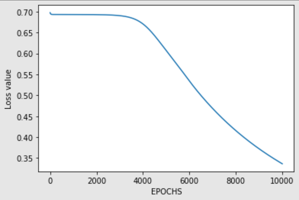

Let us define the predict function through which we can utilize our trained neural network to compute some predictions. We will perform the forward propagation and squeeze the result obtained. Since we fine-tuned the weights during the training process, we should be able to achieve the desired result with a threshold of 0.5.

# Creating the predict function

def predict(w1,w2,input):
    z1, a1, z2, a2 = forward_prop(w1,w2,test)
    a2 = np.squeeze(a2)
    
    if a2>=0.5:
        print("For input", [i[0] for i in input], "output is 1")
    else:
        print("For input", [i[0] for i in input], "output is 0")

Now that we have finished defining the prediction function, we can test out the predictions made by your neural network constructed and see its performance after training the model for about 10000 iterations. We will test the results predicted for each of the four possible cases and compare them with the expected outcomes of the XOR gate.

test = np.array([[0],[0]])
predict(w1,w2,test)

test = np.array([[0],[1]])
predict(w1,w2,test)

test = np.array([[1],[0]])
predict(w1,w2,test)

test = np.array([[1],[1]])
predict(w1,w2,test)

For input [0, 0] output is 0
For input [0, 1] output is 1
For input [1, 0] output is 1
For input [1, 1] output is 0

We can notice that the results obtained after the neural network prediction are similar to the expected outcome. Hence, we can conclude that our neural network constructed from scratch is able to successfully make accurate predictions on the XOR gate task. The following GitHub reference was used for the majority of the code in this section. I would recommend checking it out if you want another resource for learning. It is also suggested that the readers try out other variations of the different types of gates by constructing neural networks from scratch to solve them.

Comparison of builds using deep learning frameworks:

The field of deep learning and artificial neural networks is vast. While it is possible to construct neural networks from scratch to solve complicated problems, it is usually not feasible due to the large amount of time required and the inherent complexity of the network that needs to be constructed. Hence, we make use of deep learning frameworks such as TensorFlow, PyTorch, MXNet, Caffe, and other similar libraries (or tools) for designing, training, and validating neural network models.

These deep learning frameworks allow the developers and researchers to quickly construct their desired models for solving a particular task without too much investment into the underlying working of intricate and unnecessary details. Out of the many deep learning frameworks that are available, two of the most popular existing tools for constructing neural networks are TensorFlow and PyTorch. In this section, we will reconstruct the project that we built in the previous sections with the help of deep learning frameworks.

For this reconstruction project, I will make use of the TensorFlow and Keras libraries. I would recommend checking out the following article to learn more about TensorFlow and the Keras article from this link (here). The code structure for this section of the article is quite simple, and you can easily reproduce it in any other deep learning framework such as PyTorch. Feel free to check out the ultimate guide to PyTorch from the following link if you want to build this project with PyTorch instead of TensorFlow. Below is the list of imports that we will use for constructing our neural network to solve AND Gate and XOR Gate.

import tensorflow as tf
from tensorflow import keras
import numpy as np

Once we have imported the necessary libraries, we can define some of the required parameters that we will utilize for constructing a neural network to learn the output of the AND Gate. Similar to the AND gate, we will also construct the XOR gate as we did in the previous section. Firstly, let us look at the construction of the AND gate. Below are the inputs and the expected outcome for the AND Gate. The logic for the AND gate is that the output is only high when both (or all) the inputs are high. Otherwise, when either of the inputs is low, the output is also low.

a = np.array([0, 0, 1, 1])
b = np.array([0, 1, 0, 1])

y_and = np.array([0, 0, 0, 1])

Once we have declared the inputs and the expected output, it is time to combine the two input arrays into a single entity. We can do this in a couple of methods, as discussed in the previous section. For this code snippet, we will append them into one list containing four separate elements, with each of the lists having two elements. The final array obtained after combining the input elements will be stored in a new array.

total_input = []

for i, j in zip(a, b):
    input1 = []
    input1.append(i)
    input1.append(j)
    total_input.append(input1)
    
total_input = np.array(total_input)

The obtained input array after the combination of the two initial input lists looks as follows.

array([[0, 0],
       [0, 1],
       [1, 0],
       [1, 1]])
       

The shape of this final input array is as follows.

(4, 2)

In the next step, we will create the training data along with their respective output labels. Firstly, we will create the lists to store the training data for both the inputs and the output. Once we finish looping through these elements, we can save these lists as arrays and use them for further computation and training with neural networks.

x_train = []
y_train = []

for i, j in zip(total_input, y_and):
    x_train.append(i)
    y_train.append(j)
    
x_train = np.array(x_train)
y_train = np.array(y_train)

The training procedure for such a task is quite simple. We can define the required libraries, namely the Input layers, the Dense layers for the hidden layers and output node, and finally, the Sequential model, so that we can construct a Sequential type model to solve the required AND gate task. Firstly, we will define the type of the model and then proceed to add the input layer, which will take the inputs as we have previously defined them. We have two hidden layers with ten nodes in each of them with the ReLU activation function. The final output layer contains the Sigmoid activation function with one node to provide us with the desired result. The final output is either zero or one, according to the provided input.

from tensorflow.keras.layers import Input, Dense
from tensorflow.keras.models import Sequential

model = Sequential()
model.add(Input(shape = x_train[0].shape))
model.add(Dense(10, activation = "relu"))
model.add(Dense(10, activation = "relu"))
model.add(Dense(1, activation = "sigmoid"))

model.summary()

Model: "sequential"
_________________________________________________________________
Layer (type)                 Output Shape              Param #   
=================================================================
dense (Dense)                (None, 10)                30        
_________________________________________________________________
dense_1 (Dense)              (None, 10)                110       
_________________________________________________________________
dense_2 (Dense)              (None, 1)                 11        
=================================================================
Total params: 151
Trainable params: 151
Non-trainable params: 0
_________________________________________________________________

The above table shows the summary of the Sequential type network containing the hidden layers and output node with their respective parameters. Now that we have constructed the model architecture to solve the required AND gate task, we can proceed to compile the model and train it accordingly. We will utilize the Adam optimizer, the binary cross-entropy loss function, and also compute the binary accuracy to verify how accurate our model is.

model.compile(optimizer = "adam", loss = "binary_crossentropy", metrics = "binary_accuracy")

Once the compilation of the model is done, let us begin the training procedure and see if the model is able to achieve the desired results. Note that contents such as loss functions and optimizers for neural networks from scratch are yet to be covered. We will cover these concepts in future articles. Below is the code snippet to train the desired model.

model.fit(x_train, y_train, epochs = 500)

We will train the model for around 500 epochs to ensure that it learns the requirements as desired. Since we have less data for these gate tasks, the model will require more training to learn and optimize the results accordingly. Once the training is complete, which should take about a few minutes, we can continue with the prediction function through which we can verify the results obtained. Let us perform the prediction on the dataset as shown in the below code snippet.

model.predict(x_train)

array([[0.00790971],
       [0.02351646],
       [0.00969902],
       [0.93897456]], dtype=float32)

We can notice that the results for the AND gate seem pretty much as expected. For output values that must be zero, the result obtained on the prediction is able to predict values close to zero, and for output values that must be one, we are getting results close to one. We can also round these values to obtain the desired result. Let us explore another gate apart from the AND gate that we just completed.

Similarly, for the XOR gate, we can also proceed to follow a similar workflow as we did for the AND gate. Firstly, we will define the required inputs for the XOR gate. It is again a 2-channel input that utilizes the variables a and b storing the input values. The y variable will store the expected result values in a NumPy array. We will combine the two input arrays similar to the method used in this section. Once the input is combined, and we get the desired combination, we will divide our data into training input information and their result label outputs.

a = np.array([0, 0, 1, 1])
b = np.array([0, 1, 0, 1])

y_xor = np.array([0, 1, 1, 0])

total_input = []

for i, j in zip(a, b):
    input1 = []
    input1.append(i)
    input1.append(j)
    total_input.append(input1)
    
total_input = np.array(total_input)

x_train = []
y_train = []

for i, j in zip(total_input, y_xor):
    x_train.append(i)
    y_train.append(j)
    
x_train = np.array(x_train)
y_train = np.array(y_train)

We will use a similar Sequential type architecture as we did earlier in this section of the article. The code snippet and the resulting summary of the model are as shown below.

model1 = Sequential()
model1.add(Input(shape = x_train[0].shape))
model1.add(Dense(10, activation = "relu"))
model1.add(Dense(10, activation = "relu"))
model1.add(Dense(1, activation = "sigmoid"))

model1.summary()

Model: "sequential_1"
_________________________________________________________________
Layer (type)                 Output Shape              Param #   
=================================================================
dense_3 (Dense)              (None, 10)                30        
_________________________________________________________________
dense_4 (Dense)              (None, 10)                110       
_________________________________________________________________
dense_5 (Dense)              (None, 1)                 11        
=================================================================
Total params: 151
Trainable params: 151
Non-trainable params: 0
_________________________________________________________________

We will define the parameters such as the optimizer and loss functions for compiling the model and then fit the model. For the training procedure, we will use the second model and the new training data inputs and outputs for the training process. We will train our model for a thousand epochs before getting the optimal predictions. The training should take only a few minutes as there are relatively few data samples to train.

model1.compile(optimizer = "adam", loss = "binary_crossentropy", metrics = "binary_accuracy")

model1.fit(x_train, y_train, epochs = 1000)

Let us perform the prediction on the training input data and look at the outputs the model is able to predict after the training procedure is complete.

model1.predict(x_train)

array([[0.01542357],
       [0.995468  ],
       [0.99343044],
       [0.00554709]], dtype=float32)

We can notice that the output values are quite accurate to the respective expected outcomes. The values are closer to zero when the expected outcome is zero, and the values are closer to one when the expected outcome is one. Finally, let us round off the values for both the predictions by both the models of the AND gate and XOR gate, respectively. Doing this step will help us achieve single integer values, as required by the expected output.

model.predict(x_train).round()
model1.predict(x_train).round()

array([[0.],
       [0.],
       [0.],
       [1.]], dtype=float32)

array([[0.],
       [1.],
       [1.],
       [0.]], dtype=float32)

We can notice that both the models trained are able to generate desirable outputs with the provided inputs. Even though we have lesser amounts of data, over a long period of training, the model is able to achieve the desired results with the reduction of the loss. To learn the working of all the essentials of neural networks from scratch is quite lengthy. The complex concepts such as optimizers, loss functions, various loss functions, and other similar topics will be covered in future articles on constructing neural networks from scratch.

Conclusion:

In this article, we showed most of the basic concepts for constructing neural networks from scratch. After a brief introduction, we explored some of the necessary elements required to understand how artificial neural networks work. Once we walked through the elementary topics, we proceeded to construct neural networks from scratch using NumPy. We experimented with the XOR gate and built an ANN that could tackle this problem. Finally, we also learned how to construct solutions to numerous gates such as AND and XOR with the help of deep learning frameworks, namely TensorFlow and Keras.

Artificial Neural Networks (ANN) and deep learning are a revolution that has the capabilities to achieve some of the most complex tasks that were once deemed to be impossible for machines to achieve. The journey of successful AI and neural networks starts with humble beginnings, from simple perceptron models to complicated n-hidden layer architecture builds. With the advent of GPUs and widespread access to affordable compute, creating such models and frameworks is becoming more and more accessible to anyone with the interest to learn how. The complexities and concepts of neural networks are numerous, especially when we are trying to construct these networks from scratch, as we did in this article. In future parts, we will explore more of the essential necessities of building neural networks from scratch.

In the upcoming articles, we will look at more variations of generative adversarial networks such as pix-2-pix GAN, BERT transformers, and of course, the second part of constructing neural networks from scratch. Until then, keep exploring and learning new stuff!