Decision Trees are the foundation for many classical machine learning algorithms like Random Forests, Bagging, and Boosted Decision Trees. They were first proposed by Leo Breiman, a statistician at the University of California, Berkeley. His idea was to represent data as a tree where each internal node denotes a test on an attribute (basically a condition), each branch represents an outcome of the test, and each leaf node (terminal node) holds a class label.
Decision trees are now widely used in many applications for predictive modeling, including both classification and regression. Sometimes decision trees are also referred to as CART, which is short for Classification and Regression Trees. Let’s discuss in-depth how decision trees work, how they're built from scratch, and how we can implement them in Python.
In this article, we'll cover the following modules:
- Why Decision Trees?
- Types of Decision Trees
- Key Terminology
- How To Create a Decision Tree
- Gini Impurity
- Chi-Square
- Information Gain
- Applications of Decision Trees
- Decoding the Hyperparameters
- Coding the Algorithm
- Advantages and Disadvantages
- Summary and Conclusion
Bring this project to life
Why Decision Trees?
Tree-based algorithms are a popular family of related non-parametric and supervised methods for both classification and regression. If you're wondering what supervised learning is, it's the type of machine learning algorithms which involve training models with data that has both input and output labels (in other words, we have data for which we know the true class or values, and can tell the algorithm what these are if it predicts incorrectly).
The decision tree looks like a vague upside-down tree with a decision rule at the root, from which subsequent decision rules spread out below. For example, a decision rule can be whether a person exercises. There can also be nodes without any decision rules; these are called leaf nodes. Before we move on, let’s quickly look into the different types of decision trees.
Types of Decision Trees
Decision Trees are classified into two types, based on the target variables.
- Categorical Variable Decision Trees: This is where the algorithm has a categorical target variable. For example, consider you are asked to predict the relative price of a computer as one of three categories: low, medium, or high. Features could include monitor type, speaker quality, RAM, and SSD. The decision tree will learn from these features and after passing each data point through each node, it will end up at a leaf node of one of the three categorical targets low, medium, or high.
- Continuous Variable Decision Trees: In this case the features input to the decision tree (e.g. qualities of a house) will be used to predict a continuous output (e.g. the price of that house).
Key Terminology
Let’s see what a decision tree looks like, and how they work when a new input is given for prediction.
Below is an image explaining the basic structure of the decision tree. Every tree has a root node, where the inputs are passed through. This root node is further divided into sets of decision nodes where results and observations are conditionally based. The process of dividing a single node into multiple nodes is called splitting. If a node doesn’t split into further nodes, then it’s called a leaf node, or terminal node. A subsection of a decision tree is called a branch or sub-tree (e.g. in the box in the image below).
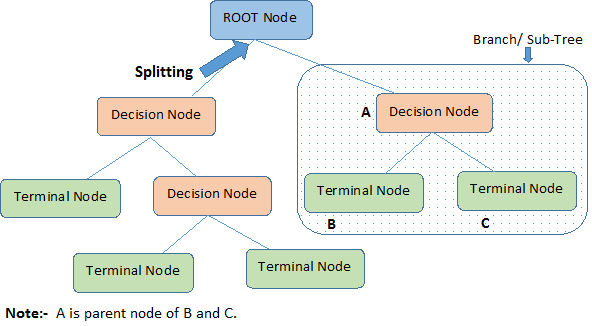
There is also another concept that is quite opposite to splitting. If there are ever decision rules which can be eliminated, we cut them from the tree. This process is known as pruning, an is useful to minimize the complexity of the algorithm.
Now that we have a clear idea of what a basic decision tree looks like, let’s dive into how the splitting is done, and how we can construct a decision tree ourselves.
How To Create a Decision Tree
In this section, we shall discuss the core algorithms describing how decision trees are created. These algorithms are completely dependent on the target variable, however, these vary from the algorithms used for classification and regression trees.
There are several techniques that are used to decide how to split the given data. The main goal of decision trees is to make the best splits between nodes which will optimally divide the data into the correct categories. To do this, we need to use he right decision rules. The rules are what directly affect the performance of the algorithm.
There are some assumptions that need to be considered before we get started:
- In the beginning, the whole data is considered as the root, thereafter, we use the algorithms to make a split or divide the root into subtrees.
- The feature values are considered to be categorical. If the values are continuous, then they are separated prior to building the model.
- Records are distributed recursively on the basis of attribute values.
- The ordering of attributes as root or internal node of the tree is done using a statistical approach.
Let’s get started with the commonly used techniques to split, and thereby, construct the Decision tree.
Gini Impurity
If all elements are correctly divided into different classes (an ideal scenario), the division is considered to be pure. The Gini impurity (pronounced like "genie") is used to gauge the likelihood that a randomly chosen example would be wrongly classified by a certain node. It is known as an "impurity" measure since it gives us an idea of how the model differs from a pure division.
The degree of the Gini impurity score is always between 0 and 1, where 0 denotes that all elements belong to a certain class (or the division is pure), and 1 denotes that the elements are randomly distributed across various classes. A Gini impurity of 0.5 denotes that the elements are distributed equally into some classes. The mathematical notation of the Gini impurity measure is given by the following formula:

Where pi is the probability of a particular element belonging to a specific class.
Now, let’s take a look at the pseudo-code for calculating and building a decision tree using the Gini Impurity measure as our guide.
Gini Index:
    for each branch in a split:
        Calculate percent branch represents  # Used for weighting
        for each class in-branch:
            Calculate the probability of that class in the given branch
            Square the class probability
        Sum the squared class probabilities
        Subtract the sum from 1  # This is the Gini Index for that branch
    Weight each branch based on the baseline probability
    Sum the weighted Gini index for each split
We'll now look at a simple example explaining the above algorithm. Consider the following table of data, where for each element (row) we have two variables describing it, and an associated class label.
| Class | Var 1 | Var 2 |
|---|---|---|
| A | 0 | 33 |
| A | 0 | 54 |
| A | 0 | 56 |
| A | 0 | 42 |
| A | 1 | 50 |
| B | 1 | 55 |
| B | 1 | 31 |
| B | 0 | -4 |
| B | 1 | 77 |
| B | 0 | 49 |
Gini Index Example:
- The baseline of the split for Var1: Var1 has 4 instances (4/10) equal to 1 and 6 instances (6/10) equal to 0.
- For Var1 == 1 & Class == A: 1 / 4 instances have class equal to A.
- For Var1 == 1 & Class == B: 3 / 4 instances have class equal to B.
- Gini Index here is 1-((1/4)^2 + (3/4)^2) = 0.375
- For Var1 == 0 & Class == A: 4 / 6 instances have class equal to A.
- For Var1 == 0 & Class == B: 2 / 6 instances have class equal to B.
- Gini Index here is 1-((4/6)^2 + (2/6)^2) = 0.4444
- We then weight and sum each of the splits based on the baseline / proportion of the data each split takes up.
- 4/10 * 0.375 + 6/10 * 0.444 = 0.41667
Information Gain
Information Gain depicts the amount of information that is gained by an attribute. It tells us how important the attribute is. Since Decision Tree construction is all about finding the right split node that assures high accuracy, Information Gain is all about finding the best nodes that return the highest information gain. This is computed using a factor known as Entropy. Entropy defines the degree of disorganization in a system. The more the disorganization is, the more is the entropy. When the sample is wholly homogeneous, then the entropy turns out to be zero, and if the sample is partially organized, say 50% of it is organized, then the entropy turns out to be one.
This acts as the base factor in determining the information gain. Entropy and Information Gain together are used to construct the Decision Tree, and the algorithm is known as ID3.
Let’s understand the step-by-step procedure that’s used to calculate the Information Gain, and thereby, construct the Decision tree,
- Calculate the entropy of the output attribute (before the split) using the formula,

Here, p is the probability of success and q is the probability of failure of the node. Say, out of the 10 data values, 5 pertain to True and 5 pertain to False, then c computes to 2, p_1 and p_2 compute to ½.
- Calculate the entropy of all the input attributes using the formula,

T is the output attribute,
X is the input attribute,
P(c) is the probability w.r.t the possible data point present at X, and
E(c) is the entropy w.r.t ‘True’ pertaining to the possible data point.
Assume an input attribute (priority) where there are two possible values mentioned, low and high. With respect to low, there are 5 data points associated, out of which, 2 pertain to True and 3 pertain to False. With respect to high, the remaining 5 data points are associated, wherein 4 pertain to True and 1 pertains to False. Then E(T, X) would be,

In E(2, 3), p is 2, and q is 3.
In E(4, 1), p is 4, and q is 1.
Compute the same repeatedly for all the input attributes in the given dataset.
- Using the above two values, calculate the Information Gain or the decrease in entropy by subtracting the entropy of each attribute from the total entropy before the split,

- Choose the attribute that has the highest information gain as the split node.
- Repeat steps 1-4 by dividing the dataset in accordance with the split. This algorithm is run until all the data is classified.
Points to remember:
- A leaf node is the one that has no entropy, or when the entropy is zero. No further splitting is done on a leaf node.
- Only the branch that needs further splitting, i.e. when the entropy > 0 (when there’s impurity) needs to undergo this splitting process.
c. Chi-Square
The chi-square method works well if the target variables are categorical like success-failure/high-low. The core idea of the algorithm is to find the statistical significance of the variations that exist between the sub-nodes and the parent node. The mathematical equation that is used to calculate the chi-square is,

It represents the sum of squares of standardized differences between the observed and the expected frequencies of the target variable.
One other main advantage of using chi-square is, it can perform multiple splits at a single node which results in more accuracy and precision.
Applications of Decision Trees
Decision Tree is one of the basic and widely-used algorithms in the fields of Machine Learning. It’s put into use across different areas in classification and regression modeling. Due to its ability to depict visualized output, one can easily draw insights from the modeling process flow. Here are a few examples wherein Decision Tree could be used,
- Business Management
- Customer Relationship Management
- Fraudulent Statement Detection
- Energy Consumption
- Healthcare Management
- Fault Diagnosis
Decoding the Hyperparameters
Scikit-learn provides some functionalities or parameters that are to be used with a Decision Tree classifier to enhance the model’s accuracy in accordance with the given data.
- criterion: This parameter is used to measure the quality of the split. The default value for this parameter is set to “Gini”. If you want the measure to be calculated by entropy gain, you can change this parameter to “entropy”.
- splitter: This parameter is used to choose the split at each node. If you want the sub-trees to have the best split, you can set this parameter to “best”. We can also have a random split for which the value “random” is set.
- max-depth: This is an integer parameter through which we can limit the depth of the tree. The default value for this parameter is set to None.
- min_samples_split: This parameter is used to define the minimum number of samples required to split an internal node.
- max_leaf_nodes: The default value of max_leaf_nodes is set to None. This parameter is used to grow a tree with max_leaf_nodes in best-first fashion.
Coding the Algorithm
Step 1: Importing the Modules
The first and foremost step in building our decision tree model is to import the necessary packages and modules. We import the DecisionTreeClassifier class from the sklearn package. This is an in-built class where the entire decision tree algorithm is coded. In this program, we shall use the iris dataset that can be imported from sklearn.datasets. The pydotplus package is used for visualizing the decision tree. Below is the code snippet,
import pydotplus
from sklearn.tree import DecisionTreeClassifier
from sklearn import datasets
Step 2: Exploring the data
Next, we make our data ready by loading it from the datasets package using the load_iris() method. We assign the data to the iris variable. This iris variable has two keys, one is a data key where all the inputs are present, namely, sepal length, sepal width, petal length, and petal width. In the target key, we have the flower type which has the values, Iris Setosa, Iris Versicolour, and Iris Virginica. We load these in the features and target variables respectively.
iris = datasets.load_iris()
features = iris.data
target = iris.target

print(features)
print(target)

Output:

[[5.1 3.5 1.4 0.2]
 [4.9 3.  1.4 0.2]
 [4.7 3.2 1.3 0.2]
 [4.6 3.1 1.5 0.2]
 [5.8 4.  1.2 0.2]
 [5.7 4.4 1.5 0.4]
. . . .
. . . .
]
[0 0 0 0 0 0 0 0 0 0 0 0 0 0 0 0 0 0 0 0 0 0 0 0 0 0 0 0 0 0 0 0 0 0 0 0 0 0 0 0 0 0 0 0 0 0 0 0 0 0 1 1 1 1 1 1 1 1 1 1 1 1 1 1 1 1 1 1 1 1 1 1 1 1 1 1 1 1 1 1 1 1 1 1 1 1 1 1 1 1 1 1 1 1 1 1 1 1 1 1 2 2 2 2 2 2 2 2 2 2 2 2 2 2 2 2 2 2 2 2 2 2 2 2 2 2 2 2 2 2 2 2 2 2 2 2 2 2 2 2 2 2 2 2 2 2 2 2 2 2]
This is how our dataset looks like.
Step 3: Create a decision tree classifier object
Here, we load the DecisionTreeClassifier in a variable named model, which was imported earlier from the sklearn package.
decisiontree = DecisionTreeClassifier(random_state=0) Step 5: Fitting the Model
This is the core part of the training process where the decision tree is constructed by making splits in the given data. We train the algorithm with features and target values that are sent as arguments to the fit() method. This method is to fit the data by training the model on features and target.
model = decisiontree.fit(features, target)Step 6: Making the Predictions
In this step, we take a sample observation and make a prediction. We create a new list comprising the flower sepal and petal dimensions. Further, we use the predict() method on the trained model to check for the class it belongs to. We can also check the probability (class probability) of the prediction by using the predict_proba method.
observation = [[ 5, 4, 3, 2]] # Predict observation's class
model.predict(observation)
model.predict_proba(observation)

Output:
array([1])
array([[0., 1., 0.]])
Step 7: Dot Data for the predictions
In this step, we export our trained model in DOT format (a graph description language). To achieve that, we use the tree class that can be imported from the sklearn package. On top of that, we use the export_graphviz method with the decision tree, features and the target variables as the parameters.
from sklearn import tree

dot_data = tree.export_graphviz(decisiontree, out_file=None,
feature_names=iris.feature_names,
class_names=iris.target_names
)
Step 8: Drawing the Graph
In the last step, we visualize the decision tree using an Image class that is to be imported from the IPython.display package.
from IPython.display import Image

graph = pydotplus.graph_from_dot_data(dot_data) # Show graph

Image(graph.create_png()) 
Advantages and Disadvantages
There are a few pros and cons that come along with the decision trees. Let’s discuss the advantages first. Decision trees take very little time in processing the data when compared to other algorithms. Few preprocessing steps like normalization, transformation, and scaling the data can be skipped. Although there are missing values in the dataset, the performance of the model won’t be affected. A Decision Tree model is intuitive and easy to explain to the technical teams and stakeholders, and can be implemented across several organizations.
Here comes the disadvantages. In decision trees, small changes in the data can cause a large change in the structure of the decision tree that in turn leads to instability. The training time drastically increases, proportional to the size of the dataset. In some cases, the calculations can go complex compared to the other traditional algorithms.
Summary and Conclusion
In this article, we’ve discussed in-depth the Decision Tree algorithm. It’s a supervised learning algorithm that can be used for both classification and regression. The primary goal of decision tree is to split the dataset as a tree based on a set of rules and conditions. We discussed the key components of a decision tree like the root node, leaf nodes, sub-trees, splitting, and pruning. Further, we’ve seen how a decision tree works and how strategic splitting is performed using popular algorithms like GINI, Information Gain, and Chi-Square. Furthermore, we used scikit-learn to code decision trees from scratch on the IRIS data set. Lastly, we discussed the advantages and disadvantages of using decision trees. There is still a lot more to learn, and this article will give you a quick-start to explore other advanced classification algorithms.