The Random Forest algorithm is one of the most popular machine learning algorithms that is used for both classification and regression. The ability to perform both tasks makes it unique, and enhances its wide-spread usage across a myriad of applications. It also assures high accuracy most of the time, making it one of the most sought-after classification algorithms. Random Forests are comprised of Decision Trees. The more trees it has, the more sophisticated the algorithm is. It selects the best result out of the votes that are pooled by the trees, making it robust. Let’s look into the inner details about the working of a Random Forest, and then code the same in Python using the scikit-learn library.
Bring this project to life
In this article we'll learn about the following modules:
- Why Random Forest?
- Disadvantages of Decision Trees
- Birth of Random Forest
- A Real-Time Example
- Difference Between Decision Trees and Random Forests
- Applications of Random Forests
- Excavating and Understanding the Logic
- Random Forest, Piece by Piece
- Computing the Feature Importance (Feature Engineering)
- Decoding the Hyperparameters
- Coding the Algorithm
- Advantages and Disadvantages
- Summary and Conclusion

Why Random Forest?
Random Forest is a Supervised Machine Learning classification algorithm. In supervised learning, the algorithm is trained with labeled data that guides you through the training process. The main advantage of using a Random Forest algorithm is its ability to support both classification and regression.
As mentioned previously, random forests use many decision trees to give you the right predictions. There’s a common belief that due to the presence of many trees, this might lead to overfitting. However, it doesn’t seem like a hindrance because only the best prediction (most voted) would be picked from amongst the possible output classes, thus ensuring smooth, reliable, and flexible executions. Now, let’s see how Random Forests are created and how they’ve evolved by overcoming the drawbacks present in decision trees.
Disadvantages of Decision Trees
A decision tree is a classification model that formulates some specific set of rules that indicates the relations among the data points. We split the observations (the data points) based on an attribute such that the resulting groups are as different as possible, and the members (observations) in each group are as similar as possible. In other words, the inter-class distance needs to be low and the intra-class distance needs to be high. This is accomplished using a variety of techniques such as Information Gain, Gini Index, etc.
There are a few discrepancies that can obstruct the fluent implementation of decision trees, including:
- Decision trees might lead to overfitting when the tree is very deep. As the decisions to split the nodes progress, every attribute is taken into consideration. It tries to be perfect in order to fit all the training data accurately, and therefore learns too much about the features of the training data and reduces its ability to generalize.
- Decision trees are greedy and are prone to finding locally optimal solutions rather than considering the globally optimal ones. At every step, it uses some technique to find the optimal split. However, the best node locally might not be the best node globally.
To overcome such problems, Random Forest comes to the rescue.
Birth of Random Forest
Creating an ensemble of these trees seemed like a remedy to solve the above disadvantages. Random Forest was first proposed by Tin Kam Ho at Bell Laboratories in 1995.
A large number of trees can over-perform an individual tree by reducing the errors that usually arise whilst considering a single tree. When one tree goes wrong, the other tree might perform well. This is an added advantage that comes along, and this ensemble formed is known as the Random Forest.
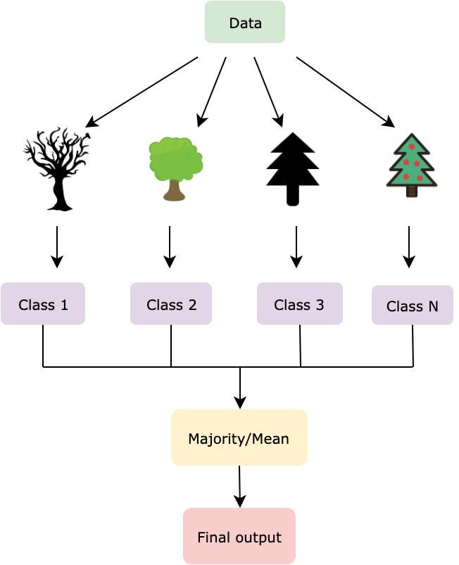
The randomly split dataset is distributed among all the trees wherein each tree focuses on the data that it has been provided with. Votes are collected from every tree, and the most popular class is chosen as the final output, this is for classification. In regression, an average is taken over all the outputs and is considered as the final result.
Unlike Decision Trees, where the best performing features are taken as the split nodes, in Random Forest, these features are selected randomly. Only a selected bag of features are taken into consideration, and a randomized threshold is used to create the Decision tree.
The algorithm is an extension of Bagging. In the Bagging technique, several subsets of data are created from the given dataset. These datasets are segregated and trained separately. In Random Forest, along with the division of data, the features are also divided, and not all features are used to grow the trees. This technique is known as feature bagging. Each tree has its own set of features allocated to it.
A Real-time example
Consider a case where you would like to build a website with one particular theme out of the options available to you. Say, you contacted a friend of yours to comment on the same and you decide to go forward with it. However, this result is biased towards the one decision that you would depend upon and doesn’t explore various other possibilities. This is where the Decision Tree is used. If at all you consulted a few people regarding the same and asked them to vote for the best theme, the bias incurred previously wouldn’t be observed here. This is because the most recommended theme is preferred to the one and the only option available in the former case. This seems like a less-biased and most reliable output and is the typical Random Forest approach. In the next section, let’s look into the differences between Decision Trees and Random Forests.
Difference between Decision Trees and Random Forests
Unlike a Decision Tree that generates rules based on the data given, a Random Forest classifier selects the features randomly to build several decision trees and averages the results observed. Also, the overfitting problem is fixed by taking several random subsets of data and feeding them to various decision trees.
Yet, Decision Tree is computationally faster in comparison to Random Forest because of the ease in generating rules. In a Random Forest classifier, several factors need to be considered to interpret the patterns among the data points.
Applications of Random Forests
Random Forest classifier is used in several applications spanning across different sectors like banking, medicine, e-commerce, etc. Due to the accuracy of its classification, its usage has increased over the years.
- Identification of the customers’ behaviors.
- Remote sensing.
- Examining the stock market trends.
- Identifying the pathologies by finding out the common patterns.
- Classifying the fraudulent and non-fraudulent actions.
Excavating and Understanding the logic
As any Machine Learning algorithm, Random Forest also consists of two phases, training and testing. One is the forest creation, and the other is the prediction of the results from the test data fed into the model. Let’s also look at the math that forms the backbone of the pseudocode.
Random Forest, piece by piece
Training: For b in 1, 2, … B, (B is the number of decision trees in a random forest)
- Firstly, apply bagging to generate random subsets of data. Given the training dataset, X and Y, bagging is done by sampling with replacement, n training examples from X, Y, by denoting them as, X_b and Y_b.
- Randomly select N features out of the total features provided.
- Calculate the best split node n from the N features.
- Split the nodes using the split point considered.
- Repeat the above 3 steps until l nodes are generated.
- Repeat the above 4 steps until B number of trees are generated.
- Testing: After the training phase is done, predict the output on the unseen samples, x’ by averaging the outputs from all the regression trees,
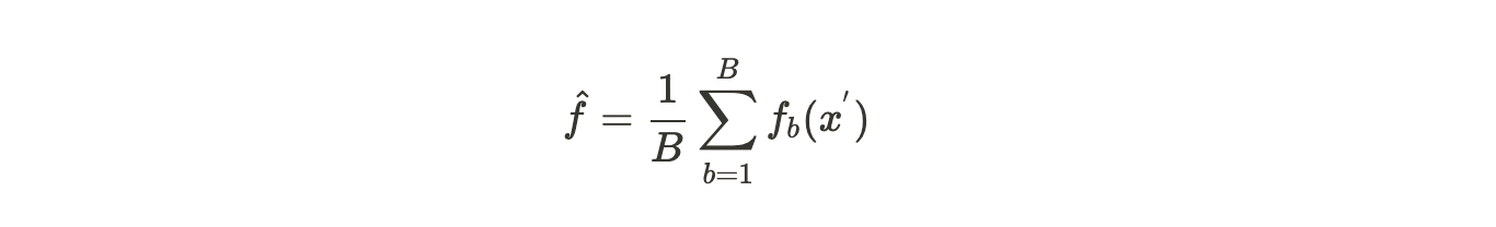
or in the case of classification, collect the votes from every tree, and consider the most voted class as the final prediction.
An optimal number of trees in a Random Forest (B) can be chosen based on the size of the dataset, cross-validation or out-of-bag error. Let’s understand these terms.
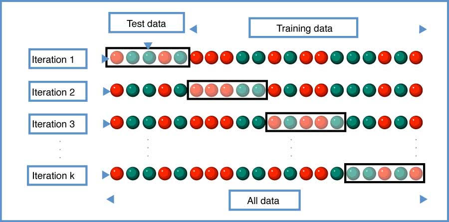
Cross-validation is generally used to reduce overfitting in machine learning algorithms. It takes training data and tests it with various test data sets across multiple iterations denoted by k, hence the name k-fold cross-validation. This can tell us the number of trees based on the k value.
Out-of-bag error is the mean prediction error on each training sample x_i, using only those trees that do not have x_i in their bootstrap sample. It’s similar to a leave-one-out-cross-validation method.
Computing the feature importance (Feature Engineering)
From here on, let’s understand how Random Forest is coded using the scikit-learn library in Python.
Firstly, measuring the feature importance gives a better overview of what features actually affect the predictions. Scikit-learn provides a good feature indicator denoting the relative importance of all the features. This is calculated using the Gini Index or Mean decrease in impurity (MDI) that measures how much the tree nodes that use that feature decrease impurity across all the trees in a forest.
It depicts the contribution made by every feature in the training phase and scales all the scores such that it sums up to 1. This, in turn, helps in shortlisting the important features and dropping the ones that don’t make a huge impact (no impact or less impact) on the model building process. The reason behind considering only a few features is to reduce overfitting that usually materializes when there is a good deal of attributes.
Decoding the hyperparameters
Scikit-learn provides some functionalities or parameters that are to be used with a Random Forest classifier to enhance the model’s speed and accuracy.
- n_estimators: It indicates the number of trees in a Random Forest. Greater the number of trees, more stable and reliable is the result that consumes higher computational power. The default value is 10 in version 0.20 and 100 in version 0.22.
- criterion: Function that measures the quality of the split (Gini/entropy). The default value is gini.
- max_depth: The maximum depth of the tree. This continues until all the leaves are pure. The default value is None.
- max_features: Number of features to look for at each split. Default value is auto, i.e. sqrt(number_of_features).
- min_samples_leaf: The minimum number of samples to be present at the leaf node. The default value is 1.
- n_jobs: The number of jobs to run in parallel for both fit and predict functions. The default value is None, i.e. only 1 job.
- oob_score: Whether to use OOB (out-of-bag) sampling to enhance generalization accuracy. The default value is False.
Coding the algorithm
Step 1: Exploring the data
Firstly, from the datasets library in sklearn package, import the MNIST data.
from sklearn import datasets

mnist = datasets.load_digits()
X = mnist.data
Y = mnist.target
Then explore the data by printing the data (input) and target (output) of the dataset.
Output:

[[ 0.  0.  5. 13.  9.  1.  0.  0.  0.  0. 13. 15. 10. 15.  5.  0.  0.  3.
  15.  2.  0. 11.  8.  0.  0.  4. 12.  0.  0.  8.  8.  0.  0.  5.  8.  0.
   0.  9.  8.  0.  0.  4. 11.  0.  1. 12.  7.  0.  0.  2. 14.  5. 10. 12.
   0.  0.  0.  0.  6. 13. 10.  0.  0.  0.]]
[0]
The input has 64 values, indicating that there are 64 attributes in the data, and the output class label is 0. To prove the same, observe the shapes of X and y wherein the data and target are stored.
print(mnist.data.shape)
print(mnist.target.shape)

Output:

(1797, 64)
(1797,)
There are 1797 data rows and 64 attributes in the dataset.
Step 2: Preprocessing the data
This step includes creating a DataFrame using Pandas. Both the target and data and stored in y and X variables respectively. pd.Series is used to fetch a 1D array of int datatype. These are a limited set of values that fall under the category data. pd.DataFrame converts the data into a tabular set of values. head() returns the top five values of the DataFrame. Let’s print them.
import pandas as pd

y = pd.Series(mnist.target).astype('int').astype('category')
X = pd.DataFrame(mnist.data)

print(X.head())
print(y.head())

Output:

   0    1    2     3     4     5    6    7    8    9  ...    54   55   56  \
0  0.0  0.0  5.0  13.0   9.0   1.0  0.0  0.0  0.0  0.0 ...   0.0  0.0  0.0
1  0.0  0.0  0.0  12.0  13.0   5.0  0.0  0.0  0.0  0.0 ...   0.0  0.0  0.0
2  0.0  0.0  0.0   4.0  15.0  12.0  0.0  0.0  0.0  0.0 ...   5.0  0.0  0.0
3  0.0  0.0  7.0  15.0  13.0   1.0  0.0  0.0  0.0  8.0 ...   9.0  0.0  0.0
4  0.0  0.0  0.0   1.0  11.0   0.0  0.0  0.0  0.0  0.0 ...   0.0  0.0  0.0

    57   58    59    60    61   62   63
0  0.0  6.0  13.0  10.0   0.0  0.0  0.0
1  0.0  0.0  11.0  16.0  10.0  0.0  0.0
2  0.0  0.0   3.0  11.0  16.0  9.0  0.0
3  0.0  7.0  13.0  13.0   9.0  0.0  0.0
4  0.0  0.0   2.0  16.0   4.0  0.0  0.0

[5 rows x 64 columns]
0    0
1    1
2    2
3    3
4    4
dtype: category
Categories (10, int64): [0, 1, 2, 3, ..., 6, 7, 8, 9]
Segregate the input (X) and the output (y) into train and test data using train_test_split imported from the model_selection package present under sklearn. test_size indicates that 70% of the data points come under training data and 30% come under testing data.
from sklearn.model_selection import train_test_split

X_train, X_test, y_train, y_test = train_test_split(X, y, test_size=0.3)
X_train is the input in the training data.
X_test is the input in the testing data.
y_train is the output in the training data.y_test is the output in the testing data.
Step 3: Creating the Classifier
Train the model on the training data using the RandomForestClassifier fetched from the ensemble package present in sklearn. n_estimators parameter indicates that a 100 trees are to be included in the Random Forest. fit() method is to fit the data by training the model on X_train and y_train.
from sklearn.ensemble import RandomForestClassifier

clf=RandomForestClassifier(n_estimators=100)
clf.fit(X_train,y_train)
Predict the outputs using predict() method applied on the X_test data. This gives the predicted values that would be stored in y_pred.
y_pred=clf.predict(X_test)Check for the accuracy using accuracy_score method imported from metrics package present in sklearn. The accuracy is estimated against both the actual values (y_test) and the predicted values (y_pred).
from sklearn.metrics import accuracy_score

print("Accuracy: ", accuracy_score(y_test, y_pred))

Output:

Accuracy:  0.9796296296296296
This gives 97.96% as the estimated accuracy of the trained Random Forest classifier. A good score indeed!
Step 4: Estimating the feature importance
In the previous sections, feature importance has been mentioned as an important characteristic of the Random Forest Classifier. Let’s compute that now.
feature_importances_ is provided by the sklearn library as part of the RandomForestClassifier. Extract and then sort the values in descending order to first print the values that are the most significant.
feature_imp=pd.Series(clf.feature_importances_).sort_values(ascending=False)
print(feature_imp[:10])

Output:

21    0.049284
43    0.044338
26    0.042334
36    0.038272
33    0.034299
dtype: float64
The left column denotes the attribute label, i.e. 26th attribute, 43rd attribute, and so on, and the right column is the number indicating the feature importance.
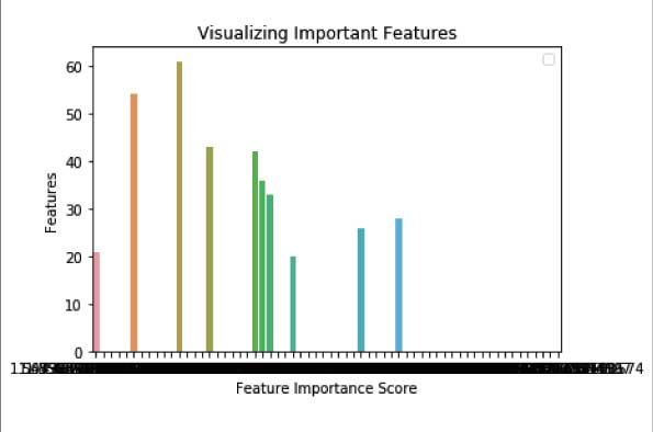
Step 5: Visualizing the feature importance
Import the libraries matplotlib.pyplot and seaborn to visualize the above feature importance outputs. Give the input and output values wherein x is given by the feature importance values, and y is the 10 most significant features out of the 64 attributes respectively.
import matplotlib.pyplot as plt
import seaborn as sns

%matplotlib inline
sns.barplot(x=feature_imp, y=feature_imp[:10].index)
plt.xlabel('Feature Importance Score')
plt.ylabel('Features')
plt.title("Visualizing Important Features")
plt.legend()
plt.show()
Advantages and Disadvantages
While it can be used for both classification and regression, Random Forest has an edge over other algorithms in the following ways,
- It is a robust and versatile algorithm.
- It can be used to handle missing values in the given data.
- It can be used to solve unsupervised ML problems.
- Understanding the algorithm is a cakewalk.
- Default hyperparameters used to give a good prediction.
- Solves the overfitting problem.
- It can be used as a feature selection tool.
- It handles high dimensional data well.
A few downsides go hand in hand with the advantages,
- It is computationally expensive.
- It is difficult to interpret.
- A large number of trees takes an ample of time.
- Creating predictions is often quite slow.
Summary and Conclusion
Random Forest’s simplicity, diversity, robustness, and reliability trump the alternative algorithms available. It offers a lot of scope in improving the model’s precision by tuning the hyperparameters and choosing the crucial features.
This article starts off by describing how a Decision Tree often acts as a stumbling block, and how a Random Forest classifier comes to the rescue. Moving on, the differences and real-time applications are explored. Later, the pseudocode is broken down into various phases by simultaneously exploring the math flavor in it. Hands-on coding experience is delivered in the following section.
There’s a lot more in store, and Random Forest is one way of tackling a machine-learning solvable problem.
References
https://towardsdatascience.com/understanding-random-forest-58381e0602d2
https://syncedreview.com/2017/10/24/how-random-forest-algorithm-works-in-machine-learning/
https://builtin.com/data-science/random-forest-algorithm
https://www.datacamp.com/community/tutorials/random-forests-classifier-python
https://en.wikipedia.org/wiki/Random_forest
https://en.wikipedia.org/wiki/Out-of-bag_error
https://scikit-learn.org/stable/modules/generated/sklearn.ensemble.RandomForestClassifier.html