This article gives a review of the Faster R-CNN model developed by a group of researchers at Microsoft. Faster R-CNN is a deep convolutional network used for object detection, that appears to the user as a single, end-to-end, unified network. The network can accurately and quickly predict the locations of different objects. In order to truly understand Faster R-CNN, we must also do a quick overview of the networks that it evolved from, namely R-CNN and Fast R-CNN.
The article starts by quickly reviewing the region-based CNN (R-CNN), which is the first trial towards building an object detection model that extracts features using a pre-trained CNN. Next, Fast R-CNN is quickly reviewed, which is faster than the R-CNN but unfortunately neglects how the region proposals are generated. This is later solved by the Faster R-CNN, which builds a region-proposal network that can generate region proposals that are fed to the detection model (Fast R-CNN) to inspect for objects.
The outline of this article is as follows:
- Overview of the Object Detection Pipeline
- R-CNN Review
- Fast R-CNN Overview
- Faster R-CNN
- Main Contributions
- Region Proposal Network (RPN)
- Anchors
- Objectness Score
- Feature Sharing between RPN and Fast R-CNN
- Training Faster R-CNN
- Alternating Training
- Approximate Joint Training
- Non-Approximate Joint Training
- Drawbacks
- Mask R-CNN
- Conclusion
- References
The papers mentioned in the article are available to download for free. The citations and links to download these papers are available at the end of this article in the References section.
Let's get started.
Bring this project to life
Overview of the Object Detection Pipeline
Traditional object detection techniques follow the 3 major steps given in the figure below. The first step involves generating several region proposals. These region proposals are candidates that might have objects within them. The number of these regions is usually in the several thousands, e.g. 2,000 or more. Examples of some algorithms that generate region proposals are Selective Search and EdgeBoxes.
From each region proposal, a fixed-length feature vector is extracted using various image descriptors like the histogram of oriented gradients (HOG), for example. This feature vector is critical to the success of the object detectors. The vector should adequately describe an object even if it varies due to some transformation, like scale or translation.
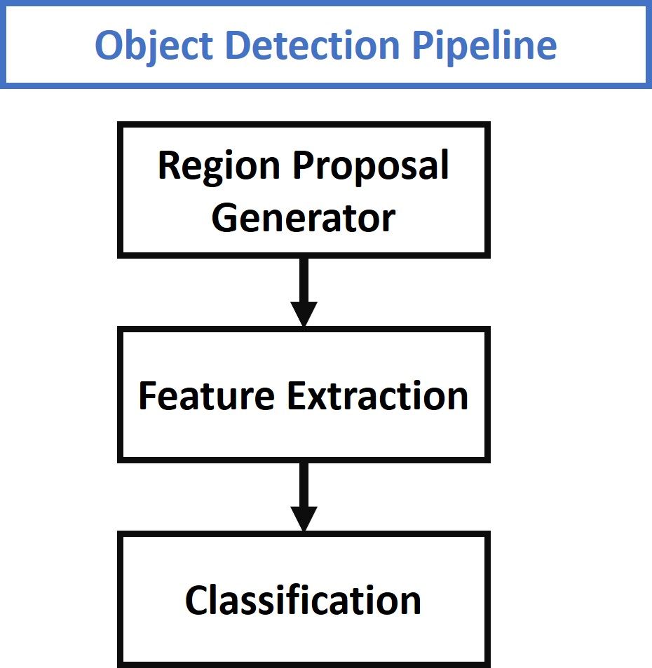
The feature vector is then used to assign each region proposal to either the background class or to one of the object classes. As the number of classes increases, the complexity of building a model that can differentiate between all of these objects increases. One of the popular models used for classifying the region proposals is the support vector machine (SVM).
This quick overview is enough to understand the basics of the region-based convolutional neural network (R-CNN).
R-CNN Quick Overview
In 2014, a group of researchers at UC Berkely developed a deep convolutional network called R-CNN (short for region-based convolutional neural network) $[1]$ that can detect 80 different types of objects in images.
Compared to the generic pipeline of the object detection techniques shown in the previous figure, the main contribution of R-CNN $[1]$ is just extracting the features based on a convolutional neural network (CNN). Other than this, everything is similar to the generic object detection pipeline. The next figure shows the working of the R-CNN model.
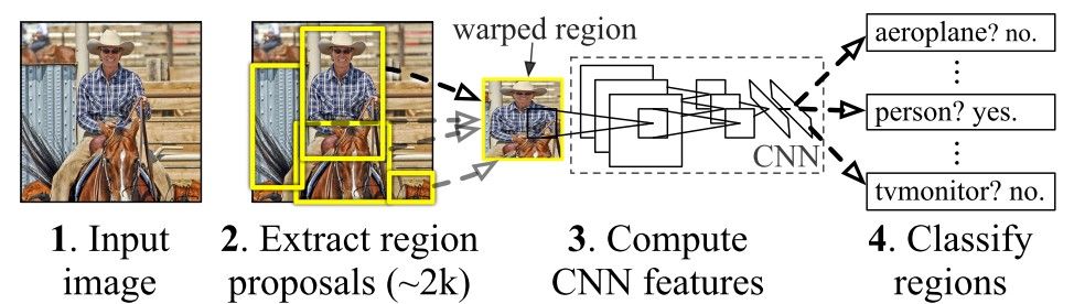
The R-CNN consists of 3 main modules:
- The first module generates 2,000 region proposals using the Selective Search algorithm.
- After being resized to a fixed pre-defined size, the second module extracts a feature vector of length 4,096 from each region proposal.
- The third module uses a pre-trained SVM algorithm to classify the region proposal to either the background or one of the object classes.
The R-CNN model has some drawbacks:
- It is a multi-stage model, where each stage is an independent component. Thus, it cannot be trained end-to-end.
- It caches the extracted features from the pre-trained CNN on the disk to later train the SVMs. This requires hundreds of gigabytes of storage.
- R-CNN depends on the Selective Search algorithm for generating region proposals, which takes a lot of time. Moreover, this algorithm cannot be customized to the detection problem.
- Each region proposal is fed independently to the CNN for feature extraction. This makes it impossible to run R-CNN in real-time.
As an extension of the R-CNN model, the Fast R-CNN model is proposed $[2]$ to overcome some limitations. A quick overview of Fast R-CNN is given in the next section.
Fast R-CNN Quick Overview
Fast R-CNN $[2]$ is an object detector that was developed solely by Ross Girshick, a Facebook AI researcher and a former Microsoft Researcher. Fast R-CNN overcomes several issues in R-CNN. As its name suggests, one advantage of the Fast R-CNN over R-CNN is its speed.
Here is a summary of the main contributions in $[2]$:
- Proposed a new layer called ROI Pooling that extracts equal-length feature vectors from all proposals (i.e. ROIs) in the same image.
- Compared to R-CNN, which has multiple stages (region proposal generation, feature extraction, and classification using SVM), Faster R-CNN builds a network that has only a single stage.
- Faster R-CNN shares computations (i.e. convolutional layer calculations) across all proposals (i.e. ROIs) rather than doing the calculations for each proposal independently. This is done by using the new ROI Pooling layer, which makes Fast R-CNN faster than R-CNN.
- Fast R-CNN does not cache the extracted features and thus does not need so much disk storage compared to R-CNN, which needs hundreds of gigabytes.
- Fast R-CNN is more accurate than R-CNN.
The general architecture of Fast R-CNN is shown below. The model consists of a single-stage, compared to the 3 stages in R-CNN. It just accepts an image as an input and returns the class probabilities and bounding boxes of the detected objects.
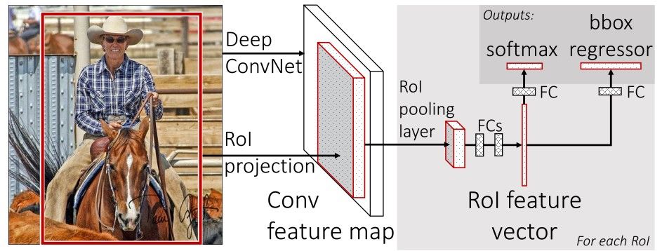
The feature map from the last convolutional layer is fed to an ROI Pooling layer. The reason is to extract a fixed-length feature vector from each region proposal. The GIF below shows how the ROI Pooling layer works.
Simply put, the ROI Pooling layer works by splitting each region proposal into a grid of cells. The max pooling operation is applied to each cell in the grid to return a single value. All values from all cells represent the feature vector. If the grid size is 2×2, then the feature vector length is 4.
For more information about the ROI Pooling layer, check out this article.
The extracted feature vector using the ROI Pooling is then passed to some FC layers. The output of the last FC layer is split into 2 branches:
- Softmax layer to predict the class scores
- FC layer to predict the bounding boxes of the detected objects
In R-CNN, each region proposal is fed to the model independently from the other region proposals. This means that if a single region takes S seconds to be processed, then N regions take S*N seconds. The Fast R-CNN is faster than the R-CNN as it shares computations across multiple proposals.
R-CNN $[1]$ samples a single ROI from each image, compared to Fast R-CNN $[2]$ that samples multiple ROIs from the same image. For example, R-CNN selects a batch of 128 regions from 128 different images. Thus, the total processing time is 128*S seconds.
For Faster R-CNN, the batch of 128 regions may be selected from just 2 images (64 regions per image). When regions are sampled from the same image, then their convolutional layer computations are shared, and this reduces the time. So, the processing time drops to 2*S. However, sampling multiple regions from the same image degrades the performance as all regions are correlated.
Despite the advantages of the Fast R-CNN model, there is a critical drawback as it depends on the time-consuming Selective Search algorithm to generate region proposals. The Selective Search method cannot be customized on a specific object detection task. Thus, it may not be accurate enough to detect all target objects in the dataset.
In the next section, Faster R-CNN $[3]$ is introduced. Faster R-CNN builds a network for generating region proposals.
Faster R-CNN
Faster R-CNN $[3]$ is an extension of Fast R-CNN $[2]$. As its name suggests, Faster R-CNN is faster than Fast R-CNN thanks to the region proposal network (RPN).
Main Contributions
The main contributions in this paper are $[3]$:
- Proposing region proposal network (RPN) which is a fully convolutional network that generates proposals with various scales and aspect ratios. The RPN implements the terminology of neural network with attention to tell the object detection (Fast R-CNN) where to look.
- Rather than using pyramids of images (i.e. multiple instances of the image but at different scales) or pyramids of filters (i.e. multiple filters with different sizes), this paper introduced the concept of anchor boxes. An anchor box is a reference box of a specific scale and aspect ratio. With multiple reference anchor boxes, then multiple scales and aspect ratios exist for the single region. This can be thought of as a pyramid of reference anchor boxes. Each region is then mapped to each reference anchor box, and thus detecting objects at different scales and aspect ratios.
- The convolutional computations are shared across the RPN and the Fast R-CNN. This reduces the computational time.
The architecture of Faster R-CNN is shown in the next figure. It consists of 2 modules:
- RPN: For generating region proposals.
- Fast R-CNN: For detecting objects in the proposed regions.
The RPN module is responsible for generating region proposals. It applies the concept of attention in neural networks, so it guides the Fast R-CNN detection module to where to look for objects in the image.
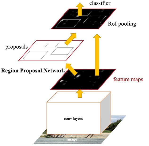
Note how the convolutional layers (e.g. computations) are shared across both the RPN and the Fast R-CNN modules.
The Faster R-CNN works as follows:
- The RPN generates region proposals.
- For all region proposals in the image, a fixed-length feature vector is extracted from each region using the ROI Pooling layer $[2]$.
- The extracted feature vectors are then classified using the Fast R-CNN.
- The class scores of the detected objects in addition to their bounding-boxes are returned.
Region Proposal Network (RPN)
The R-CNN and Fast R-CNN models depend on the Selective Search algorithm for generating region proposals. Each proposal is fed to a pre-trained CNN for classification. This paper $[3]$ proposed a network called region proposal network (RPN) that can produce the region proposals. This has some advantages:
- The region proposals are now generated using a network that could be trained and customized according to the detection task.
- Because the proposals are generated using a network, this can be trained end-to-end to be customized on the detection task. Thus, it produces better region proposals compared to generic methods like Selective Search and EdgeBoxes.
- The RPN processes the image using the same convolutional layers used in the Fast R-CNN detection network. Thus, the RPN does not take extra time to produce the proposals compared to the algorithms like Selective Search.
- Due to sharing the same convolutional layers, the RPN and the Fast R-CNN can be merged/unified into a single network. Thus, training is done only once.
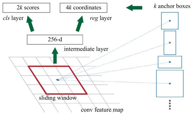
The RPN works on the output feature map returned from the last convolutional layer shared with the Fast R-CNN. This is shown in the next figure. Based on a rectangular window of size nxn, a sliding window passes through the feature map. For each window, several candidate region proposals are generated. These proposals are not the final proposals as they will be filtered based on their "objectness score" (explained below).
Anchor
According to the next figure, the feature map of the last shared convolution layer is passed through a rectangular sliding window of size nxn, where n=3 for the VGG-16 net. For each window, K region proposals are generated. Each proposal is parametrized according to a reference box which is called an anchor box. The 2 parameters of the anchor boxes are:
- Scale
- Aspect Ratio
Generally, there are 3 scales and 3 aspect ratios and thus there is a total of K=9 anchor boxes. But K may be different than 9. In other words, K regions are produced from each region proposal, where each of the K regions varies in either the scale or the aspect ratio. Some of the anchor variations are shown in the next figure.
Using reference anchors (i.e. anchor boxes), a single image at a single scale is used while being able to offer scale-invariant object detectors, as the anchors exist at different scales. This avoids using multiple images or filters. The multi-scale anchors are key to share features across the RPN and the Fast R-CNN detection network.
For each nxn region proposal, a feature vector (of length 256 for ZF net and 512 for the VGG-16 net) is extracted. This vector is then fed to 2 sibling fully-connected layers:
- The first FC layer is named
cls, and represents a binary classifier that generates the objectness score for each region proposal (i.e. whether the region contains an object, or is part of the background). - The second FC layer is named
regwhich returns a 4-D vector defining the bounding box of the region.
The first FC layer (i.e. binary classifier) has 2 outputs. The first is for classifying the region as a background, and the second is for classifying the region as an object. The next section discusses how the objectness score is assigned to each anchor and how it is used to produce the classification label.
Objectness Score
The cls layer outputs a vector of 2 elements for each region proposal. If the first element is 1 and the second element is 0, then the region proposal is classified as background. If the second element is 1 and the first element is 0, then the region represents an object.
For training the RPN, each anchor is given a positive or negative objectness score based on the Intersection-over-Union (IoU).
The IoU is the ratio between the area of intersection between the anchor box and the ground-truth box to the area of union of the 2 boxes. The IoU ranges from 0.0 to 1.0. When there is no intersection, the IoU is 0.0. As the 2 boxes get closer to each other, the IoU increases until reaching 1.0 (when the 2 boxes are 100% identical).
The next 4 conditions use the IoU to determine whether a positive or a negative objectness score is assigned to an anchor:
- An anchor that has an IoU overlap higher than 0.7 with any ground-truth box is given a positive objectness label.
- If there is no anchor with an IoU overlap higher than 0.7, then assign a positive label to the anchor(s) with the highest IoU overlap with a ground-truth box.
- A negative objectness score is assigned to a non-positive anchor when the IoU overlap for all ground-truth boxes is less than 0.3. A negative objectness score means the anchor is classified as background.
- Anchors that are neither positive nor negative do not contribute to the training objective.
I was confused by the second and third conditions when I was first reading the paper. So, let's give more clarification.
Assume there are 3 region proposals associated with 3 anchors, where their IoU scores with 3 ground-truth boxes are listed below. Because there is an anchor with an IoU score of 0.9, which is higher than 0.7, it is assigned a positive objectness score with that ground-truth box, and negative to all other boxes.
0.9, 0.55, 0.1Here is the result of classifying the anchors:
positive, negative, negativeThe second condition means that when no anchor has an IoU overlap score higher than 0.7, then search for the anchor with the highest IoU and assign it a positive objectness score. It is expected that the maximum IoU score is less than or equal to 0.7, but the confusing part is that the paper did not mention a minimum value of the IoU score.
It is expected that the minimum value should be 0.5. So, if an anchor box has an IoU score that is greater than 0.5 but less than or equal to 0.7, then assign it a positive objectness score.
Assume that the IoU scores of an anchor are listed below. Because the highest IoU score is the second one with a value of 0.55, it falls under the second condition. Thus, it is assigned a positive objectness score.
0.2, 0.55, 0.1Here is the result of classifying the anchors:
negative, positive, negativeThe third condition specifies that when the IoU scores of an anchor with all ground-truth boxes are less than 0.3, then this anchor is assigned a negative objectness score. For the next IoU scores, the anchor is given a negative score for the 3 cases because all of the IoU scores are less than 0.3.
0.2, 0.25, 0.1Here is the result of classifying the anchors:
negative, negative, negativeAccording to the fourth condition, when an anchor has an IoU score that is greater than or equal to 0.3 but less than or equal to 0.5, it is neither classified as positive nor negative. This anchor is not used in training the classifier.
For the following IoU scores the anchor is not assigned any label, as all of the scores are between 0.3 and 0.5 (inclusive).
0.4, 0.43, 0.45The next equation summarizes the 4 conditions.
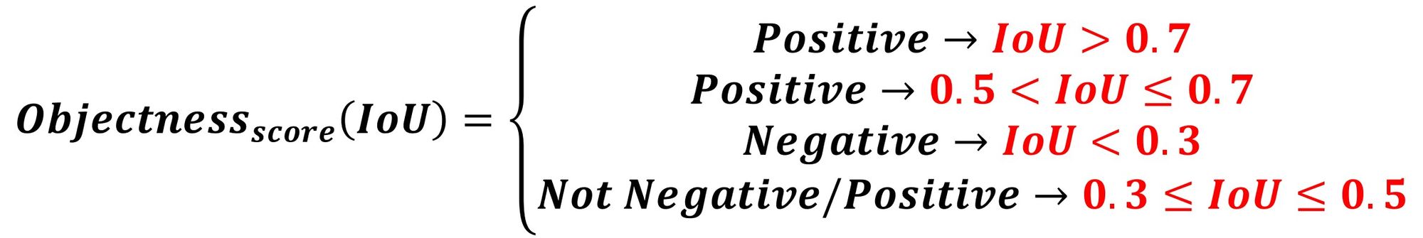
Note that the first condition (0.7 < IoU) is usually sufficient to label an anchor as positive (i.e. contains an object) but the authors preferred to mention the second condition (0.5 < IoU <= 0.7) for the rare cases where there is no region with an IoU of 0.7.
Feature Sharing between RPN and Fast R-CNN
The 2 modules in the Fast R-CNN architecture, namely the RPN and Fast R-CNN, are independent networks. Each of them can be trained separately. In contrast, for Faster R-CNN it is possible to build a unified network in which the RPN and Fast R-CNN are trained at once.
The core idea is that both the RPN and Fast R-CNN share the same convolutional layers. These layers exist only once but are used in the 2 networks. It is possible to call it layer sharing or feature sharing. Remember that the anchors $[3]$ are what makes it possible to share the features/layers between the 2 modules in the Faster R-CNN.
Training Faster R-CNN
The Faster R-CNN paper $[3]$ mentioned 3 different ways to train both the RPN and Fast R-CNN while sharing the convolutional layers:
- Alternating Training
- Approximate Joint Training
- Non-Approximate Joint Training
Alternating Training
The first method is called alternating training, in which the RPN is first trained to generate region proposals. The weights of the shared convolutional layers are initialized based on a pre-trained model on ImageNet. The other weights of the RPN are initialized randomly.
After the RPN produces the boxes of the region proposals, the weights of both the RPN and the shared convolutional layers are tuned.
The generated proposals by the RPN are used to train the Fast R-CNN module. In this case, the weights of the shared convolutional layers are initialized with the tuned weights by the RPN. The other Fast R-CNN weights are initialized randomly. While the Fast R-CNN is trained, both the weights of Fast R-CNN and the shared layers are tuned. The tuned weights in the shared layers are again used to train the RPN, and the process repeats.
According to $[3]$, alternating training is the preferred way to train the 2 modules and is applied in all experiments.
Approximate Joint Training
The second method is called approximate joint training, in which both the RPN and Fast R-CNN are regarded as a single network, not 2 separate modules. In this case, the region proposals are produced by the RPN.
Without updating the weights of neither the RPN nor the shared layers, the proposals are fed directly to the Fast R-CNN which detects the objects' locations. Only after the Fast R-CNN produces its outputs are the weights in the Faster R-CNN tuned.
Because the weights of the RPN and the shared layers are not updated after the region proposals are generated, the weights' gradients with respect to the region proposals are ignored. This reduces the accuracy of this method compared to the first method (even if the results are close). On the other hand, the training time is reduced by about 25-50%.
Non-Approximate Joint Training
In the approximate joint training method, an RoI Warping layer is used to allow the weights' gradients with respect to the proposed bounding boxes to be calculated.
Drawbacks
One drawback of Faster R-CNN is that the RPN is trained where all anchors in the mini-batch, of size 256, are extracted from a single image. Because all samples from a single image may be correlated (i.e. their features are similar), the network may take a lot of time until reaching convergence.
Mask R-CNN
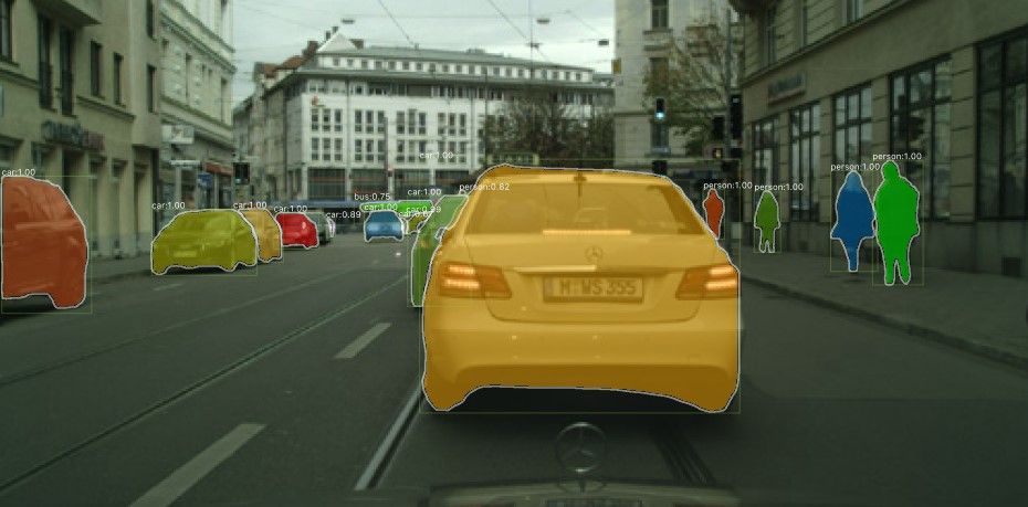
As an extension to Faster R-CNN $[3]$, the Mask R-CNN model includes another branch that returns a mask for each detected object.
Conclusion
This article reviewed a deep convolutional neural network used for object detection called Faster R-CNN, which accurately detects and classifies objects in images.
The article started by reviewing the generic steps of any object detection model. It then quickly reviewed how the R-CNN and Fast R-CNN models work in order to have an idea of what challenges Faster R-CNN is conquering.
Faster R-CNN is a single-stage model that is trained end-to-end. It uses a novel region proposal network (RPN) for generating region proposals, which save time compared to traditional algorithms like Selective Search. It uses the ROI Pooling layer to extract a fixed-length feature vector from each region proposal.
One drawback we saw of Faster R-CNN is that for the RPN, all anchors in the mini-batch are extracted from a single image. Because all samples from a single image may be correlated (i.e. their features are similar), the network may take a lot of time until reaching convergence.
That being said, Faster R-CNN is a state of the art object detection model. Mask R-CNN has since been built off of Faster R-CNN to return object masks for each detected object.
References
- Girshick, Ross, et al. "Rich feature hierarchies for accurate object detection and semantic segmentation." Proceedings of the IEEE conference on computer vision and pattern recognition. 2014.
- Girshick, Ross. "Fast r-cnn." Proceedings of the IEEE international conference on computer vision. 2015.
- Ren, Shaoqing, et al. "Faster r-cnn: Towards real-time object detection with region proposal networks." Advances in neural information processing systems. 2015.
- He, Kaiming, et al. "Mask r-cnn." Proceedings of the IEEE international conference on computer vision. 2017.