Component-based research in computer vision has accelerated significantly over the recent years, especially with the advent of adversarial attacks and attention mechanisms. One of the primary components which has been extensively revived over the recent period is that of the non-linear transformation layers, known as activation functions. Although activation functions may be considered somewhat trivial in the grand scheme of the current landscape of research, their contribution to the training dynamics of modern neural networks in all fields of deep learning is massive and undeniable.
In this post we will do an in-depth analysis into one of the most recently proposed form of activation functions published at the 16th European Conference on Computer Vision, 2020 (ECCV). Titled "Funnel Activation for Visual Recognition", the paper introduces a novel activation in the rectified non-linearities family known as FReLU.
This article is divided into four sections. Firstly, we will go over a brief prior to activation functions in general, especially into the rectified non-linear functions family. Next, we will go in-depth into the novel FReLU, and the intuition and theory behind the paper. Further, we will discuss the results presented in the paper and conclude by analyzing the potential shortcomings of the idea, and areas for improvement or further study.
You can run the associated code for this article for free on the ML Showcase.
Bring this project to life
Table of Contents:
- Activation Functions
- ReLU family
- Recent advancements in non-linearities
- Funnel Activation
- Code
- Results
- Shortcomings
- References
Activation Functions
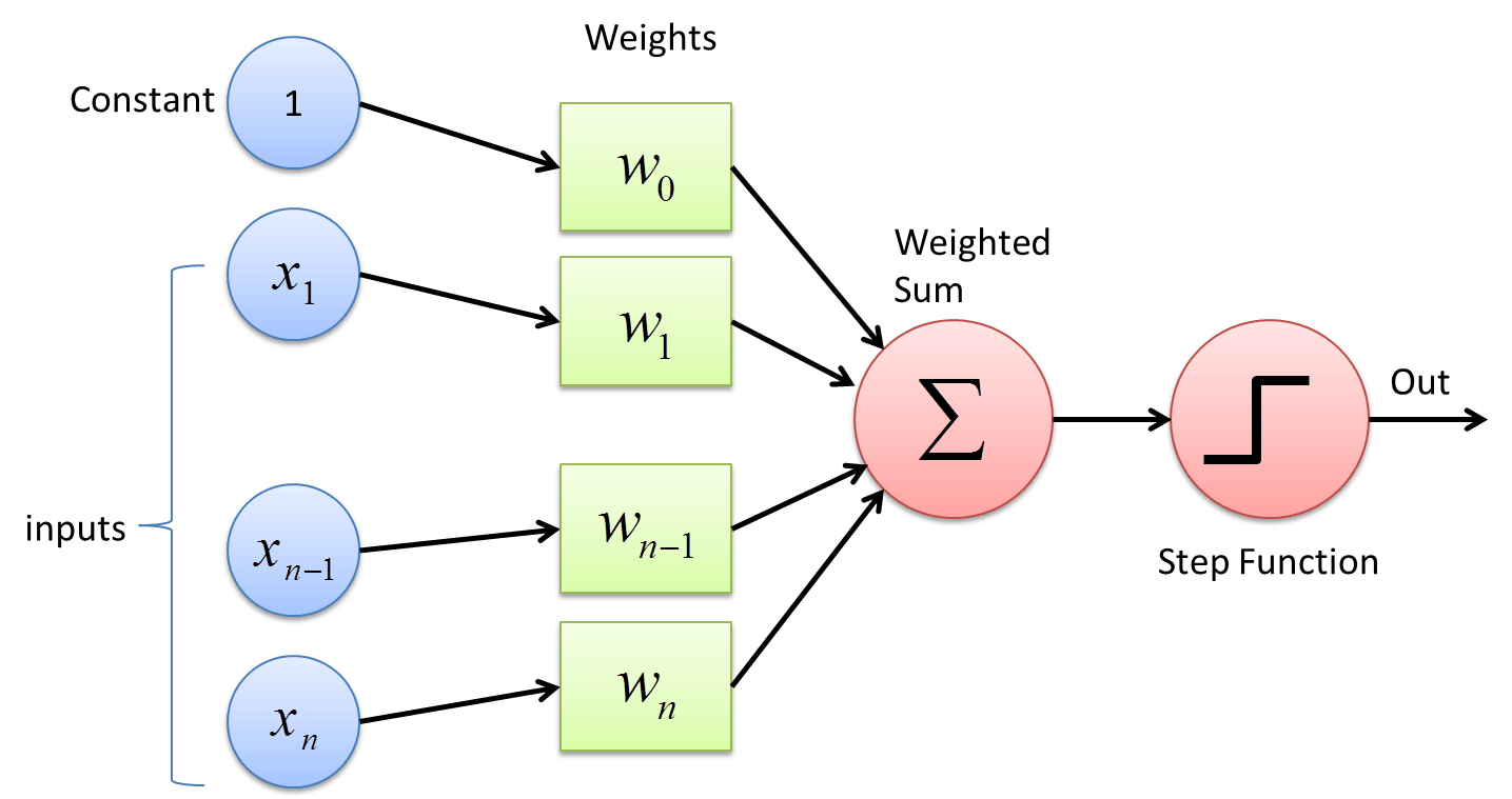
Activation functions are a crucial factor in the training dynamics of neural networks. They serve the purpose of introducing non-linearity into the network. It all started with a simple step function in the perceptron, where the output of the step function was binary (either 1 or 0). This gave the notion of whether the information propagated by the neurons preceding it was important enough to fire/activate that neuron (imagine it to be similar to a switch). However, this caused a huge loss in information and was soon replaced by a smoother alternative which helped in gradient backpropagation: the sigmoid function.
Later, the use of Rectified Linear Units (ReLU) became more standardized after the release of the paper "Rectified Linear Units Improve Restricted Boltzmann Machines" in 2010. It has been a decade since and there have been countless new forms of activation functions, however, ReLU has still reigned supreme owing to their versatility in different deep learning tasks and their computational efficiency.
Recent advancements in understanding the importance of activation functions have led to the exploration of smoother variants which improve both the generalization capability and the robustness of the deep neural network. Some of the most prominent examples of this include:
- Swish (Searching for Activation Functions)
- GELU (Gaussian Error Linear Units)
- Mish (Mish: A Self Regularized Non-Monotonic Activation Function)
ReLU Family
As discussed in the previous section, ReLU has been the long-standing faithful non-linearity for most deep learning or machine learning practitioners and researchers. However, ReLU has some distinct disadvantages which have been addressed by different forms of ReLU, like Leaky ReLU and PReLU. We will include these activation functions in the ReLU family because they all have the form of a piecewise linear function with mostly the negative half of the function distinctly different, as compared to the standard ReLU.
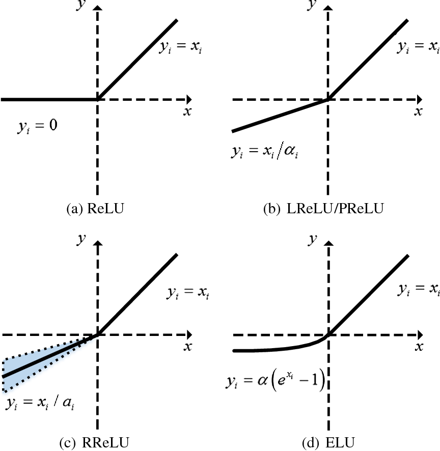
Firstly, let's understand the shortcomings of ReLU. ReLU is a simple piecewise linear function of the form $y(x) = \max(0,x)$. Hence, it thresholds all negative components of the input signal to zero. This causes a massive loss of potentially useful information. While there are other disadvantages of using ReLU, we will only use the thresholding property to build our discussion on FReLU, since it has served as the fundamental motivation for other forms of ReLU.
To tackle this issue, Leaky ReLU was introduced as a potential fix. Leaky ReLU introduced a non-zero negative half of the function by modulating the negative components of the input signal by a small pre-determined scalar value, denoted as $\alpha$ (usually 0.01). Thus, the function takes the form of $\max(\alpha x, x)$. Although this proved to be a success, the intuition behind using a predefined value to condition the slope of the negative half of the function gave way for a more fundamentally correct, learnable form of Leaky ReLU known as Parametric ReLU (PReLU).
The functional forms of PReLU and Leaky ReLU are the same, however, the only caveat is that the $\alpha$ is now a learnable parameter and is not predefined. This therefore helps the network to learn a stable and good slope for the negative half of the function, and removes the discrepancy of hard-coding it. This will form the basis of understanding the motivation for FReLU.
For the scope of this review article, we won't be covering other activation functions in the ReLU family like RReLU, Smooth ReLU, ELU, etc.
Recent Advancements In Non-Linearities
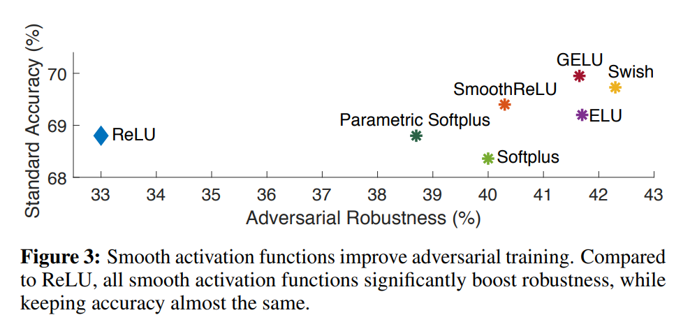
The role of the activation function has also been recently extended to incorporate the adversarial robustness of a neural network, with smoother activation functions providing better robustness than the same network equipped, for instance, with vanilla ReLU. This was explored in a recent paper titled Smooth Adversarial Training.
Smooth functions have mostly been investigated from the point of view of a pointwise scalar transformation, where the most successful and popular options combine existing functions into a composite structure to form smoother alternatives like Mish ( $f(x) = x\tanh(\log(1+e^{x}))$ ) and Swish ( $f(x)=xsigmoid(\beta x)$ ).
However, there have been other dimensions of exploration as well. Let's do a brief case study on those types using the exact terminologies that the paper used.
Contextual Conditional Activations
As the name suggests, contextual conditional activations are those non-linear transformations which are conditioned by the context, and thus are many-to-one functions. One of the most prominent examples of this type of activation function is the Maxout function. Defined as $max(\omega_{1}^{T}x + b_{1},\omega_{2}^{T}x + b_{2})$, it basically makes the layer a dual/multi-branch structure and selects the max child node of the two, unlike other pointwise scalar activation functions which are applied directly on the dot product of the weights and the input, which is represented as: $\psi(x)=f(\omega^{T}x + b)$. Thus, Maxout networks incorporate both ReLU and Leaky ReLU/ PReLU structures into the same framework.
Gating
Mostly introduced by Language Modeling with Gated Convolutional Networks, these activations are mostly composite or product functions where one of the sub-functions is gated by another functional transformation of the input, or the raw input itself.
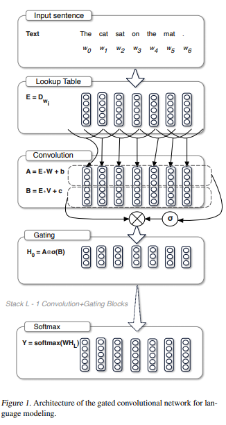
As shown, in an RNN-based structure, we have two sets of input to the activation function post-convolution, represented as A and B. The activation of choice here is sigmoid, represented as $\sigma(x) = \frac{1}{1+e^{-x}}$. Thus, the gating activation is of the form $H_{0}= A \bigotimes \sigma(B)$. Thus, here the activation $\sigma(B)$ is gated by A. The idea of gating was later extended to vision by Sigmoid-Weighted Linear Units for Neural Network Function Approximation in Reinforcement Learning, where the authors introduced Sigmoid-Weighted Linear Units (SiLU) which can be approximated to $f(x)=xsigmoid(x)$. Here the only twist is that, instead of a different input being used for gating, the same input which is passed to the non-linear function is used as the gate. This form of gating was then appropriately named "self-gating". This was later on validated by Searching for Activation Functions, where the authors used a NAS approach to find Swish defined as $f(x) = xsigmoid(\beta x)$. This basically introduced a simple trainable parameter in the form of $\beta$ to add more flexibility and adaptive nature during training.
The idea of self-gating can be on a very abstract level related to the role of skip connections, where the non-modulated input is used as a controlled update of the output of a block of convolutional layers. Skip connections form the foundation of Residual Networks, and it has been evidently proven that skip connections make the optimization contour of the network much smoother and thus easier to optimize and results in better generalization and improved robustness.
There are more examples of recent proposals of smooth activation functions which employ self gating, like that of:
- GELU (Gaussian Error Linear Units): $f(x)=x\frac{1}{2}[1+erf(x/\sqrt{2})]$
- Mish (Mish: A Self Regularized Non-Monotonic Activation Function): $f(x)=x\tanh(softplus(x))$
Continuing on contextual conditional activation functions, these were more relevant in RNN-based structures because the sequence length was much smaller compared to the input space in image domains, where a 4-D tensor of B × C × H × W dimensions can have a huge number of input data points. This is the reason why most context-conditioned activation functions are only channel conditioned. However, the authors argue that spatial conditioning is equally as important as channel adaptive conditioning. To address the increased computational requirements, FReLU incorporates depthwise-separable convolution kernels (DWConv) of 3×3 window size by default, which is extremely cheap in terms of parameters and FLOPs.
Spatial Dependency Modelling
Although spatial adaptive activation functions were not elaboratively explored earlier, the goal of introducing spatial adaptive modeling isn't new and isn't derived from activation functions. The goal of spatial dependency modeling was more discussed in the context of attention mechanisms, where capturing long-range dependencies is crucial. For example, Global Context Networks (GCNet) (see GCNet: Non-local Networks Meet Squeeze-Excitation Networks and Beyond), a form of Non-Local Networks (NLNet) (see Non-local Neural Networks) uses a variant of channel attention to capture long-range dependencies.
Additionally, to capture non-linear spatial dependencies, at different ranges convolutional kernels of different sizes have been used to aggregate feature representation. However, this is not as efficient as it adds more parameters and operations. Comparatively, FReLU solves these issues by introducing a cheap module that allows computing activation while capturing spatial dependencies and not introducing any add-on module.
Subsequently, FReLU is able to apply non-linear transformation for individual pixels by using adaptive receptive fields using simple efficient DWConv, rather than using complex convolution operators to introduce variable receptive fields depending on the input, which is known to improve the performance of deep convolutional neural networks (CNN).
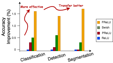
Because of ticking all these properties, FReLU is able to perform better than other activation functions by a considerable margin consistently in different domains of image recognition and transfer learning, as shown by the plot below:
Funnel Activation
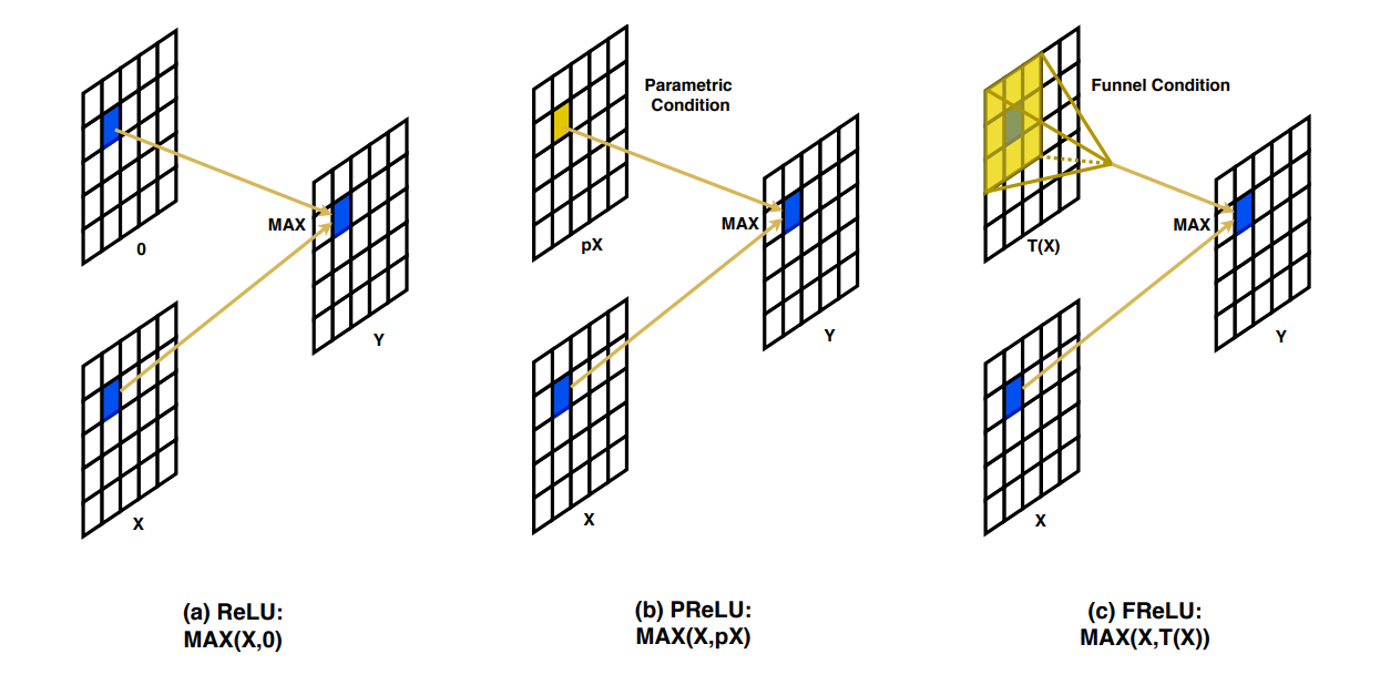
As discussed earlier, ReLU is a piecewise linear function. However, it can be interpreted as a conditional pointwise scalar operation applied for every point (pixel) of the input. The condition is a max function and the two operands are the pixel in question and zero. Thus, every negative-valued point is changed to zero.
To fix this, and to additionally make Leaky ReLU more powerful, parametric ReLU (PReLU) was introduced. PReLU aims at keeping the same conditional operation, except the comparative value was that of a parametric scaled input, where the scalar parameter was learned during training. As visualized above, essentially, while computing the activation for a given pixel x, compare it using the max operation with the same pixel scaled by a learnable scalar value $\alpha$. This thus helps in preserving negative information and reducing information loss, and improves signal propagation through the depth of the neural network.
The downside to this is that the learnable scalar $\alpha$ is disjointed from the contextual representation of the input. This is where FReLU, or Funnel Activation, provides an easy fix. Instead of learning a single fixed scalar value, it learns an aggregated representation of the local neighborhood around the target pixel and uses that as the comparative value in the max operation. This learned aggregated representation of the local context is represented as a function defined as $\mathbb{T}(x)$. Thus, the equation for FReLU becomes $f(x) = \max(x, \mathbb{T}(x))$. The spatial conditional dependency function $\mathbb{T}(x)$ is defined as a Parametric Pooling Window and is of the size $k × k$, and is always centered on the target pixel.
The Parametric Pooling Window in its functional form can be mathematically defined as:
$\mathbb{T}(x_{c,i,j}^{\omega}) = x_{c,i,j}^{\omega} \circ x_{c}^{\omega}$
Where c denotes the channel index for that pixel; i, j denotes the spatial co-ordinates of that pixel in that channel; and p is the coefficient for that window per channel c. Thus, the parametric pooling window function is essentially a channel-wise dot product of the input with a coefficient.
The authors use gaussian initialization to initialize the coefficients to have initial conditions to keep values close to zero. This approximates ReLU because $\mathbb{T}(x) \approx 0$ is approximating $\max(x, 0)$ which is the definition of ReLU. The authors report in their paper that they investigated non-parametric methods of aggregation like average pool and max-pool. They observed the performance to be comparatively worse than the parametric form, thus justifying the increase in model weights by involving a parametric form of aggregation.
Thus, in a nutshell, the parametric pooling window is essentially a depthwise convolution kernel defined by the size k × k, where k is set to 3 by default. This is followed by a batch normalization layer. Thus, for an input tensor of dimension C × H × W, the amount of extra parameters introduced by FReLU is equal to C × k × k, and since k <<< C, the order of additional complexity introduced is equivalent to the number of channels in the input tensor.
Code
The authors provide the official implementation for FReLU based on the MegEngine framework.
You can also run the Jupyter notebook associated with this article for free from the ML Showcase.
Original Implementation
"""
To install megengine, use the following command in your terminal:
pip3 install megengine -f https://megengine.org.cn/whl/mge.html
Or if on Google Colab then:
!pip3 install megengine -f https://megengine.org.cn/whl/mge.html
"""
import megengine.functional as F
import megengine.module as M

class FReLU(M.Module):
    r""" FReLU formulation. The funnel condition has a window size of kxk. (k=3 by default)
    """
    def __init__(self, in_channels):
        super().__init__()
        self.conv_frelu = M.Conv2d(in_channels, in_channels, 3, 1, 1, groups=in_channels)
        self.bn_frelu = M.BatchNorm2d(in_channels)

    def forward(self, x):
        x1 = self.conv_frelu(x)
        x1 = self.bn_frelu(x1)
        x = F.maximum(x, x1)
        return x
PyTorch Implementation
import torch
import torch.nn as nn

class FReLU(nn.Module):
    r""" FReLU formulation. The funnel condition has a window size of kxk. (k=3 by default)
    """
    def __init__(self, in_channels):
        super().__init__()
        self.conv_frelu = nn.Conv2d(in_channels, in_channels, 3, 1, 1, groups=in_channels)
        self.bn_frelu = nn.BatchNorm2d(in_channels)

    def forward(self, x):
        x1 = self.conv_frelu(x)
        x1 = self.bn_frelu(x1)
        x = torch.max(x, x1)
        return x
Note: you can increase kernel size to be larger than 3, however, you'll have to accordingly increase the padding to keep the convolution a spatial and depth preserving one.
Results
Before looking at the comparative results of FReLU, let's first take a look at the ablation studies conducted by the authors. The authors left no stone unturned in their exploration of finding the optimal form of FReLU. We will go through experiments on type of condition, compatibility of FReLU in standard models and layers, type of normalization used, etc.
| Model | Activation | Top-1 Error |
|---|---|---|
| A | Max(x, ParamPool(x)) | 22.4 |
| B | Max(x, MaxPool(x)) | 24.4 |
| C | Max(x, AvgPool(x)) | 24.5 |
| A | Max(x, ParamPool(x)) | 22.4 |
| D | Sum(x, ParamPool(x)) | 23.6 |
| E | Max(DW(x), 0) | 23.7 |
Here, the authors validate the importance of Parametric Pooling Window $\mathbb{T}(x)$ which they use as the condition. In models B and C, they replace the Parametric Pooling Window with MaxPool and Average Pool respectively. Further, in model D, they replace the max operation with a sum operation to simulate a similar form to that of a skip connection. Lastly, in model E, they use the context condition which is computed by the depthwise-separable convolution kernel represented as DW as the operand for ReLU. They validate these settings using a ResNet-50 backbone on the ImageNet-1k dataset and confirm the Parametric Pooling Window to be superior to other variants in terms of error rate in the image classification task.
| Normalization | Top-1 Error |
|---|---|
| No Normalization | 37.6 |
| Batch Normalization | 37.1 |
| Layer Normalization | 36.5 |
| Instance Normalization | 38.0 |
| Group Normalization | 36.5 |
The authors experimented with different normalization layers in computing the spatial condition in FReLU. Note: this doesn't include the default Batch Normalization layers already present in the model without FReLU. They used the ShuffleNet v2 network for the ImageNet-1k classification task for this experiment. Although the authors found that Layer Normalization and Group Normalization achieves the lowest error, they use Batch Normalization since it doesn't have any effect on Inference speed. This question was raised in this issue in their official repository, where the authors pointed to this article for further clarification on the effect of normalization layers on inference speed.
| Model | Window size | Top-1 Error |
|---|---|---|
| A | 1×1 | 23.7 |
| B | 3×3 | 22.4 |
| C | 5×5 | 22.9 |
| D | 7×7 | 23.0 |
| E | Sum(1×3,3×1) | 22.6 |
| F | Max(1×3, 3×1) | 22.4 |
The authors further experiment on different kernel sizes starting from a pointwise convolution of size 1 × 1, to aggregating horizontal and vertical sliding windows using a sum and max function. They found the 3 × 3 kernel size to be performing best for a ResNet-50 on ImageNet-1k classification task.
| Stage 2 | Stage 3 | Stage 4 | Top-1 Error |
|---|---|---|---|
| ✓ | 23.1 | ||
| ✓ | 23.0 | ||
| ✓ | 23.3 | ||
| ✓ | ✓ | 22.8 | |
| ✓ | ✓ | 23.0 | |
| ✓ | ✓ | ✓ | 22.4 |
A ResNet is defined as a model of 4 stages in total. Each stage contains predefined numbers of bottleneck/basic blocks which contain the convolutional layers. The authors validated the importance of adding FReLU in every stage and replacing the pre-existing ReLU layers present. As shown in the above table, FReLU in all stages performs the best in ImageNet-1k classification task using a ResNet-50 network.
| 1×1 conv. | 3×3 conv. | Top-1 Error | |
|---|---|---|---|
| ResNet-50 | ✓ | 22.9 | |
| ResNet-50 | ✓ | 23.0 | |
| ResNet-50 | ✓ | ✓ | 22.4 |
| MobileNet | ✓ | 29.2 | |
| MobileNet | ✓ | 29.0 | |
| MobileNet | ✓ | ✓ | 28.5 |
To understand layer compatibility the authors observed the performance of replacing ReLU with 1×1 convolutional layers, 3×3 convolutional layers, and both 1×1 and 3×3 convolutional layers in the bottleneck structure of MobileNet and ResNet-50 with FReLU. As per the table above, replacing all ReLU with FReLU performs superior to other configurations. Note: often the 1×1 convolution layers are called channel convolution since they're responsible for changing the channel dimension of the input tensor, while the 3×3 convolutional layers are called spatial convolutional layers since they usually don't change the channel dimension of the input. Instead they are rather responsible for changing the spatial dimensions of the input.
| Model | Number of Parameters (in millions) | FLOPs | Top-1 Error |
|---|---|---|---|
| ReLU | 25.5M | 3.9G | 24.0 |
| FReLU | 25.5M | 3.9G | 22.4 |
| ReLU+SE | 26.7M | 3.9G | 22.8 |
| FReLU+SE | 26.7M | 3.9G | 22.1 |
Further, the authors verified the compatibility of FReLU with other plug-and-play accuracy-improving methods, for instance, attention mechanisms. The choice of the module here was that of a Squeeze-and-Excitation (SE) module, which is a channel attention method. The authors verified that using SE with FReLU provides the best comparative performance.
Note: we've covered Squeeze-and-Excitation Networks in our Attention Mechanisms for Computer Vision Series. You can read about it here.
Now onto the comparative benchmarks for ImageNet classification and Semantic Segmentation.
ImageNet Benchmarks on ResNets
| Model | Activation | Number of Parameters (in millions) | FLOPs | Top-1 Error |
|---|---|---|---|---|
| ResNet-50 | ReLU | 25.5M | 3.86G | 24.0 |
| ResNet-50 | PReLU | 25.5M | 3.86G | 23.7 |
| ResNet-50 | Swish | 25.5M | 3.86G | 23.5 |
| ResNet-50 | FReLU | 25.5M | 3.87G | 22.4 |
| ResNet-101 | ReLU | 44.4M | 7.6G | 22.8 |
| ResNet-101 | PReLU | 44.4M | 7.6G | 22.7 |
| ResNet-101 | Swish | 44.4M | 7.6G | 22.7 |
| ResNet-101 | FReLU | 44.5M | 7.6G | 22.1 |
ImageNet Benchmarks on Lightweight Mobile Architectures
| Model | Activation | Number of Parameters (in millions) | FLOPs | Top-1 Error |
|---|---|---|---|---|
| MobileNet 0.75 | ReLU | 2.5M | 325M | 29.8 |
| MobileNet 0.75 | PReLU | 2.5M | 325M | 29.6 |
| MobileNet 0.75 | Swish | 2.5M | 325M | 28.9 |
| MobileNet 0.75 | FReLU | 2.5M | 328M | 28.5 |
| ShuffleNetV2 | ReLU | 1.4M | 41M | 39.6 |
| ShuffleNetV2 | PReLU | 1.4M | 41M | 39.1 |
| ShuffleNetV2 | Swish | 1.4M | 41M | 38.7 |
| ShuffleNetV2 | FReLU | 1.4M | 45M | 37.1 |
Object Detection Benchmarks on MS-COCO using RetinaNet Detector
| Model | Activation | Number of Parameters (in millions) | FLOPs | mAP | AP50 | AP75 | APs | APm | APl |
|---|---|---|---|---|---|---|---|---|---|
| ResNet-50 | ReLU | 25.5M | 3.86G | 35.2 | 53.7 | 37.5 | 18.8 | 39.7 | 48.8 |
| ResNet-50 | Swish | 25.5M | 3.86G | 35.8 | 54.1 | 38.7 | 18.6 | 40.0 | 49.4 |
| ResNet-50 | FReLU | 25.5M | 3.87G | 36.6 | 55.2 | 39.0 | 19.2 | 40.8 | 51.9 |
| ShuffleNetV2 | ReLU | 3.5M | 299M | 31.7 | 49.4 | 33.7 | 15.3 | 35.1 | 45.2 |
| ShuffleNetV2 | Swish | 3.5M | 299M | 32.0 | 49.9 | 34.0 | 16.2 | 35.2 | 45.2 |
| ShuffleNetV2 | FReLU | 3.7M | 318M | 32.8 | 50.9 | 34.8 | 17.0 | 36.2 | 46.8 |
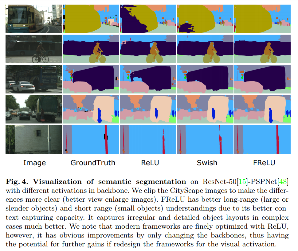
Semantic Segmentation Benchmarks on CityScapes using a PSP-Net with a Pretrained ResNet-50 Architecture
| ReLU | Swish | FReLU | |
|---|---|---|---|
| mean IU | 77.2 | 77.5 | 78.9 |
| road | 98.0 | 98.1 | 98.1 |
| sidewalk | 84.2 | 85.0 | 84.7 |
| building | 92.3 | 92.5 | 92.7 |
| wall | 55.0 | 56.3 | 59.5 |
| fence | 59.0 | 59.6 | 60.9 |
| pole | 63.3 | 63.6 | 64.3 |
| traffic light | 71.4 | 72.1 | 72.2 |
| traffic sign | 79.0 | 80.0 | 79.9 |
| vegetation | 92.4 | 92.7 | 92.8 |
| terrain | 65.0 | 64.0 | 64.5 |
| sky | 94.7 | 94.9 | 94.8 |
| person | 82.1 | 83.1 | 83.2 |
| rider | 62.3 | 65.5 | 64.7 |
| car | 95.1 | 94.8 | 95.3 |
| truck | 77.7 | 70.1 | 79.8 |
| bus | 84.9 | 84.0 | 87.8 |
| train | 63.3 | 68.8 | 74.6 |
| motorcycle | 68.3 | 69.4 | 69.8 |
| bicycle | 78.2 | 78.4 | 78.7 |
Shortcomings
- Although the results are comparatively much better, this doesn't hide the fact that DWConv is not optimized for hardware and is inefficient. The parameters and FLOPs don't reflect this, however the latency and throughput are going to be significantly worse than the vanilla model.
- FReLU is at the end a form of ReLU which isn't smooth, and as shown in the earlier sections, smooth activations tend to have a higher degree of adversarial robustness as compared to their non-smooth counterparts.
Alas, it's on the users/readers/practitioners/researchers to try FReLU on their own models and evaluate its efficiency.
References
- Funnel Activation for Visual Recognition, ECCV 2020.
- Original Repository for FReLU.
- Searching for Activation Functions
- Mish: A Self Regularized Non-Monotonic Activation Function, BMVC 2020.
- Gaussian Error Linear Units
- Language Modeling with Gated Convolutional Networks
- Wikipedia Page for Activation Functions