Global Context Networks (GCNet) Explained

Non-Local Networks have provided a strong intuition and foundation for many modern attention mechanisms used in deep neural network architectures for computer vision.

In this post we will go through one of the prominent works which took inspiration from Non-Local Networks and Squeeze-and-Excitation Networks to model an attention mechanism which enables the network to capture long-range dependencies at a considerably cheap cost. This is known as the Global Context Network, which was accepted at ICCV Workshops in 2019.

First we will revisit Non-Local Networks briefly before recapping Squeeze-and-Excitation networks. Then we will move to an in-depth discussion of Global Context Modeling, before providing its code and observing the results presented in the paper. We will finally conclude by considering some shortcomings of GCNet.

Table of Contents

• Abstract Overview
• Revisiting Non-Local Networks
• Revisiting Squeeze-and-Excitation Networks
• Global Context Networks
  • PyTorch Code
• Results
• Shortcomings
• References

Abstract Overview

However, through a rigorous empirical analysis, we have found that the global contexts modeled by non-local networks are almost the same for different query positions within an image. In this paper, we take advantage of this finding to create a simplified network based on a query independent formulation, which maintains the accuracy of NLNet but with significantly less computation. We further observe that this simplified design shares similar structure with Squeeze-Excitation Network (SENet). Hence we unify them into a three-step general framework for global context modeling. Within the general framework, we design a better instantiation, called the global context (GC) block, which is lightweight and can effectively model the global context.

Revisiting Non-Local Networks

Non-Local Networks took an impactful approach to capturing long-range dependencies, via aggregating query-specific global context to each query position. Simply put, Non-Local Networks are responsible for modeleing the attention map of a single pixel by aggregating the relational information of its surrounding pixels. It achieved this by using few permutation operations to allow the attention map to be constructed with the focal query pixel. This approach is somewhat, in an abstract sense, similar to that of the Self-Attention Mechanism proposed in SAGAN.

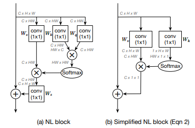
As shown in the above diagram, the NL Block essentially takes in the input tensor and first permutes it from $C \times H \times W \times C \times HW$ dimension format. This permutation is followed by three branches. In one of the branches, it simply undergoes $1 \times 1$ pointwise spatial preserving convolution. In the other two branches, it also goes through similar convolution operations but then they're multiplied by the cross product by permuting one of the outputs, after which the resultant output is passed through a SoftMax activation layer which outputs an $HW \times HW$ shaped tensor. This output is then multiplied by the cross product with the output of the first branch to give a resultant $C \times HW$ output, which is then permuted to a shape of $C \times H \times W$ before being element-wise added to the original input to the block like a residual connection.

The GCNet paper provides a simplified and generalized form of the Non-Local Block, as shown in the above diagram. The input to this simplified block is passed in parallel through two $1 \times 1$ convolution operators, where one preserves the channel and spatial dimensions while the next only reduces the channel dimension to $1$. The first convolution's output is then permuted from $C \times H times W$ to $C \times HW$, similar to the classic Non-Local Block, while the second convolution's output is reshaped from $1 \times H \times W$ to $HW \times 1 \times 1$. These two tensors are subsequently multiplied using the cross product, which results in an output tensor of the shape $C \times 1 \times 1$. This output tensor is then similarly added to the original input like a residual connection.

Revisiting Squeeze-and-Excitation Networks

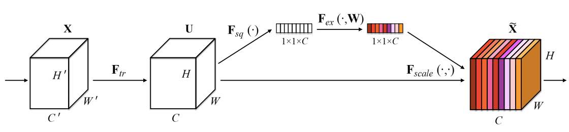
Squeeze-and-Excitation Networks incorporate a channel attention mechanism that essentially is made up of three components: a Squeeze Block, Excitation Block, and Scaling Block.

The Squeeze Block is responsible for reducing the input feature maps $(C \times H \times W)$ to single pixels using Global Average Pooling (GAP) while keeping the number of channels the same $(C \times 1 \times 1)$. The squeezed tensor is then passed to the Excitation block, which is a multi-layer perceptron bottleneck (MLP) responsible for learning the channel attention weights. Finally, these singular weights are passed through sigmoid activation and then are element-wise multiplied to their corresponding channels in the non-modulated input tensor.

To read an in-depth review of Squeeze-and-Excitation Networks, you can read my article on it here.

Global Context Networks

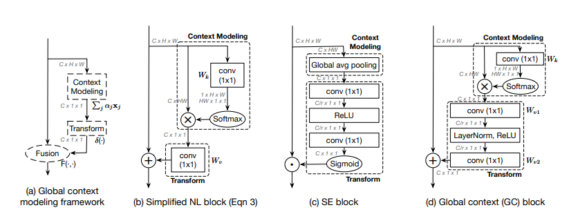
The GCNet paper proposes a unified simple module that can generalize both Squeeze-and-Excitation Networks and Non-Local Networks. This module is called the Global Context Modeling Framework, which contains three notable parts: Context Modeling, Transform, and Fusion. The Context Modeling is used to build the long-range dependencies for the query pixel while the transform usually denotes the dimensional change attributed to attention vectors in channel attention and finally Transform essentially fuses the attention vector with the original input.

As shown in the diagram above, this framework can generalize the Simplified Non-Local Block where the context modeling is responsible to capture the long-range dependencies. Similarly, in the case of Squeeze-and-Excitation Networks, the context modeling represents the decomposition of the input tensor by GAP. This is followed by the transform which constructs the attention weights, in this case, an MLP bottleneck.

Global Context Networks combine the best of the Simplified NL block and the Squeeze-and-Excitation block within the Global Context Modeling framework. The Context Modeling is the same as that present in the Simplified NL Block, while the transform is a bottleneck structure similar to that of the Squeeze-and-Excitation block, with the only difference being GCNet employs an additional LayerNorm in the bottleneck.

PyTorch Code

import torch
from torch import nn
from mmcv.cnn import constant_init, kaiming_init


def last_zero_init(m):
    if isinstance(m, nn.Sequential):
        constant_init(m[-1], val=0)
        m[-1].inited = True
    else:
        constant_init(m, val=0)
        m.inited = True


class ContextBlock2d(nn.Module):

    def __init__(self, inplanes, planes, pool, fusions):
        super(ContextBlock2d, self).__init__()
        assert pool in ['avg', 'att']
        assert all([f in ['channel_add', 'channel_mul'] for f in fusions])
        assert len(fusions) > 0, 'at least one fusion should be used'
        self.inplanes = inplanes
        self.planes = planes
        self.pool = pool
        self.fusions = fusions
        if 'att' in pool:
            self.conv_mask = nn.Conv2d(inplanes, 1, kernel_size=1)
            self.softmax = nn.Softmax(dim=2)
        else:
            self.avg_pool = nn.AdaptiveAvgPool2d(1)
        if 'channel_add' in fusions:
            self.channel_add_conv = nn.Sequential(
                nn.Conv2d(self.inplanes, self.planes, kernel_size=1),
                nn.LayerNorm([self.planes, 1, 1]),
                nn.ReLU(inplace=True),
                nn.Conv2d(self.planes, self.inplanes, kernel_size=1)
            )
        else:
            self.channel_add_conv = None
        if 'channel_mul' in fusions:
            self.channel_mul_conv = nn.Sequential(
                nn.Conv2d(self.inplanes, self.planes, kernel_size=1),
                nn.LayerNorm([self.planes, 1, 1]),
                nn.ReLU(inplace=True),
                nn.Conv2d(self.planes, self.inplanes, kernel_size=1)
            )
        else:
            self.channel_mul_conv = None
        self.reset_parameters()

    def reset_parameters(self):
        if self.pool == 'att':
            kaiming_init(self.conv_mask, mode='fan_in')
            self.conv_mask.inited = True

        if self.channel_add_conv is not None:
            last_zero_init(self.channel_add_conv)
        if self.channel_mul_conv is not None:
            last_zero_init(self.channel_mul_conv)

    def spatial_pool(self, x):
        batch, channel, height, width = x.size()
        if self.pool == 'att':
            input_x = x
            # [N, C, H * W]
            input_x = input_x.view(batch, channel, height * width)
            # [N, 1, C, H * W]
            input_x = input_x.unsqueeze(1)
            # [N, 1, H, W]
            context_mask = self.conv_mask(x)
            # [N, 1, H * W]
            context_mask = context_mask.view(batch, 1, height * width)
            # [N, 1, H * W]
            context_mask = self.softmax(context_mask)
            # [N, 1, H * W, 1]
            context_mask = context_mask.unsqueeze(3)
            # [N, 1, C, 1]
            context = torch.matmul(input_x, context_mask)
            # [N, C, 1, 1]
            context = context.view(batch, channel, 1, 1)
        else:
            # [N, C, 1, 1]
            context = self.avg_pool(x)

        return context

    def forward(self, x):
        # [N, C, 1, 1]
        context = self.spatial_pool(x)

        if self.channel_mul_conv is not None:
            # [N, C, 1, 1]
            channel_mul_term = torch.sigmoid(self.channel_mul_conv(context))
            out = x * channel_mul_term
        else:
            out = x
        if self.channel_add_conv is not None:
            # [N, C, 1, 1]
            channel_add_term = self.channel_add_conv(context)
            out = out + channel_add_term

        return out

Because of the combination of Non-Local Networks and Squeeze-and-Excitation Networks into a single unified framework, GCNet was able to capture long-range dependencies for query pixels while providing good attention representation over the global neighborhood, which allowed the network to be more robust to changes in the local spatial region.

Results

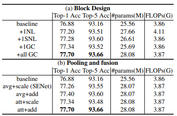
ImageNet Classification

Instance Segmentation & Object Detection on MS-COCO

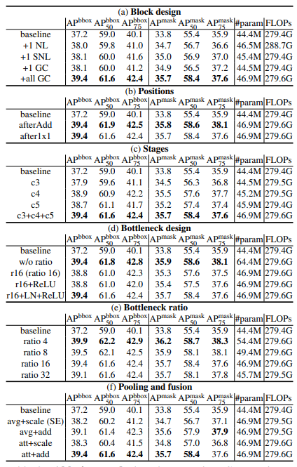
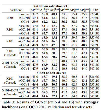
As observed, GCNet provides very strong results and considerably large performance improvements over the baseline counterpart. This is attributed to GCNet's capability to model pixel-level long-range dependencies and concurrently map channel-wise attention.

Shortcomings

1. GCNets are considerably very expensive in terms of parametric complexity. The overhead is significantly large and can be primarily attributed to the MLP bottleneck and the context modeling block, both of which add extra parameters in the order of the number of channels C, which is quite high in value.
2. Since it uses the MLP bottleneck structure employed in Squeeze-and-Excitation Networks, there is a considerable loss in information because of the dimensionality reduction in the bottleneck.

Overall, GCNet is a very strong performing attention mechanism and provides a significant gain in performance. It also received the Best Paper Award at ICCV 2019 Neural Architects Workshop.

References

1. GCNet: Non-local Networks Meet Squeeze-Excitation Networks and Beyond
2. Non-local Neural Networks
3. Squeeze-and-Excitation Networks
4. Official PyTorch implementation of GCNet
5. Self-Attention Generative Adversarial Networks