
In the first part of this series, we looked at the theory and implementation of Fourier transforms, short-time Fourier transforms, mel scale, filter banks, mel frequency cepstral coefficients, and spectral features like spectral centroid, spectral bandwidth, and spectral contrast.
Up until now, we haven't tried to understand any specific kind of sound. We took a general approach to sound analysis and how any sound looks in the frequency domain. In this article, we'll look into music in particular.
Bring this project to life
Introduction
We saw how sound travels through space in the last article. We called those waves longitudinal waves and called their fluctuations compressions and rarefactions.
Take the case of a guitar. In a guitar these final sound waves are a result of the vibrations of different guitar strings. All objects have a natural frequency with which they vibrate when struck, strummed, or are otherwise perturbed.
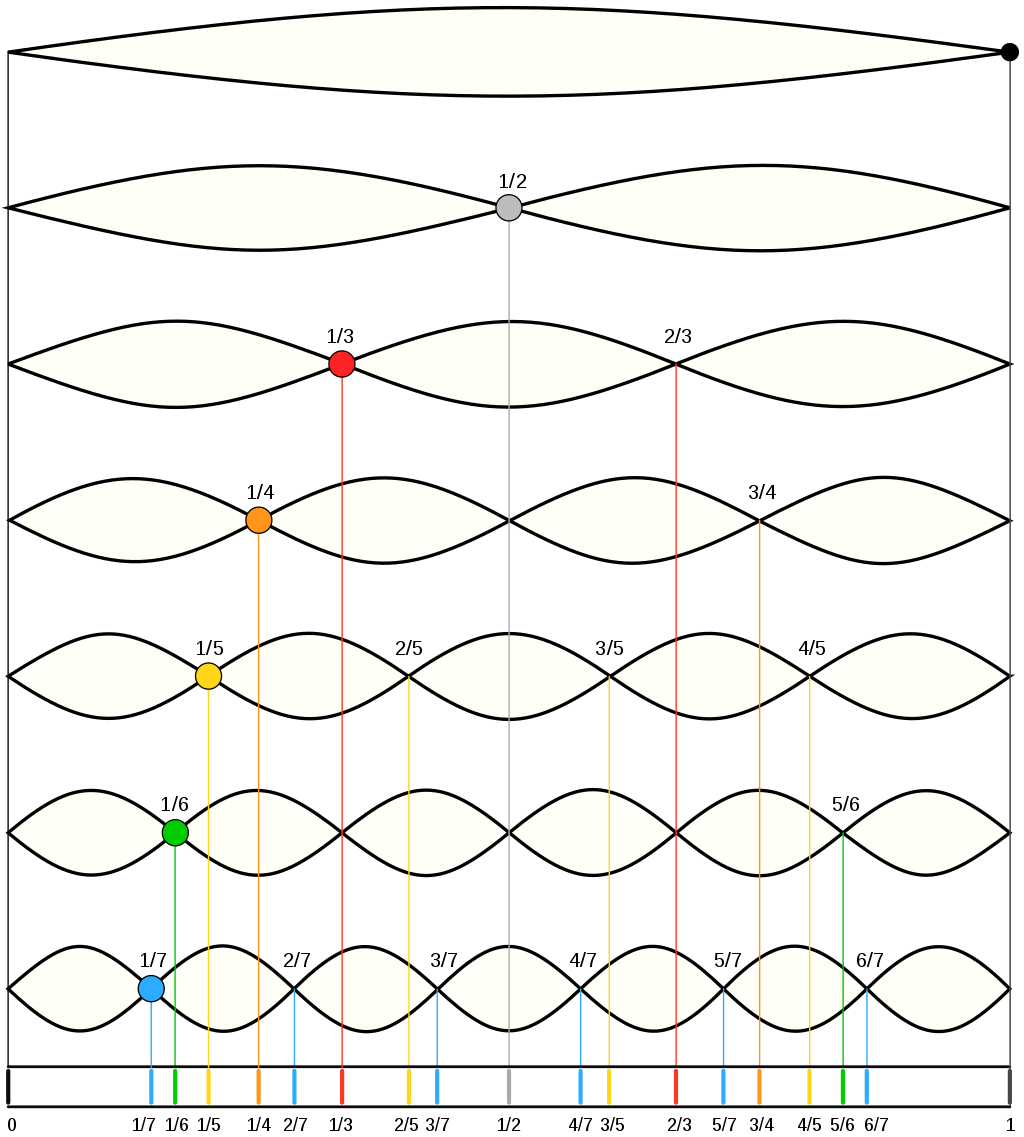
When an object is forced to vibrate in a fashion that resonates with the natural frequency, the medium tends to create what we call standing waves. Standing waves are waves that have constant amplitude profiles.
The peaks are always the same on the X-axis. So are the zero amplitude points. The points with zero amplitude show no movement at all and are called nodes.
Fundamental Frequency and Harmonics
Frequencies at which standing waves are created in a medium are referred to as harmonics. At frequencies other than harmonic frequencies, vibrations are irregular and non-repeating.
The lowest frequency produced by any particular instrument is known as the fundamental frequency or the first harmonic of the instrument. Vibrations at the fundamental frequency can be represented as a standing wave with two nodes – one at each end of the string and one anti-node at the center of the string.
The second harmonic has a frequency twice that of the first harmonic, while the third harmonic has a frequency three times that of the first harmonic. And so on and so forth.
A great animated visualization of the first four harmonics as standing waves and their longitudinal counterparts can be found here.
Notes, Octaves, and Frequencies
Certain frequencies sound pleasant to our ears when played together. Such frequencies are said to be consonant.
In music, an interval is a way of measuring the difference in the pitch of different sounds. Popular intervals in music can be represented with the following whole number ratios:
- Unison --> 1:1
- Octave --> 2:1
- Major sixth --> 5:3
- Perfect fifth --> 3:2
- Perfect fourth --> 4:3
- Major third --> 5:4
- Minor third --> 6:5
So you could say that 880Hz is an octave higher than 440Hz. Or if 440Hz is the first harmonic then 880Hz is the second harmonic.
Playing two sounds together can create interesting phenomena like beats. When two sounds of slightly different frequencies are played simultaneously, there's a periodic variation in the amplitude of the sound whose frequency is the difference between the original two frequencies.
$$ f_{beat} = f_{1} - f_{2} $$
In music, frequencies are classified into different pitch classes. In English-speaking regions, they are represented by the first 7 letters of the alphabet: A, B, C, D, E, F and G. Some might also know this as Do, Re, Mi, Fa, Sol, La and Ti, while others might know this as Sa, Re, Ga, Ma, Pa, Dha and Ni. The eighth note, or the octave, is given the same name as the first after which the pattern repeats again.
Most musical instruments today use the 12-tone chromatic scale, which divides an octave into 12 equally spaced parts on a logarithmic scale. Each part is said to be a semitone apart -- the smallest possible interval in music. Most instruments are tuned to the equally tempered scale with the note A on the middle octave tuned to 440Hz.
The 12-tone chromatic scale built on C names the 12 notes in every octave as following: C, C♯/D♭, D, D♯/E♭, E, F, F♯/G♭, G, G♯/A♭, A, A♯/B♭ and B.
♯ is pronounced as sharp and ♭ as flat. A sharp means a semitone higher while a flat means a semitone lower.
To find the frequencies in the middle octave, we need to find the frequency of the middle C. Middle C or C4's frequency is half that of C5.
Once we have have our middle C, we can create an array of size 13 that is equally spaced between the log of C4 and log of C5. We will also remove the last element (or C5 in this case) from the array.
The code is shown below:
import numpy as np

C5 = 2**np.linspace(np.log2(440), np.log2(880), 13)[3]
freqs = 2**np.linspace(np.log2(C5/2), np.log2(C5), 13)[:-1]
The resulting frequencies:
array([261.6255653 , 277.18263098, 293.66476792, 311.12698372,
       329.62755691, 349.22823143, 369.99442271, 391.99543598,
       415.30469758, 440.        , 466.16376152, 493.88330126])
Chroma Representation
A pitch can be separated into two components: tone height and chroma.
Tone height is the octave number. Middle C, for example, is also known as C4.
Chroma features, also known as chromagrams, provide a powerful way to visualize music. A chroma feature is closely related to the seven pitch classes or the twelve notes in the 12-tone chromatic scale that we just saw. A chroma representation bins all the frequencies present in a sound at any particular time into one of twelve buckets, with each bucket representing one note.
As we discussed, an octave higher than an A note is still an A even though the frequency is twice that of the previous A note. Enumerating chroma features from 0 to 11, the C note takes the index 0 and the following indices are filled by a semitone higher than the previous index.
A short time Fourier transform can be converted into a chroma representation by getting a dot product of the STFT values with chroma filters and normalizing the output.
librosa filters can be visualized using the snippet below:
chroma_filters = librosa.filters.chroma(sampling_rate, 2048)
fig, ax = plt.subplots(nrows=6, ncols=2, figsize=(12,9))

for i, row in enumerate(ax):
    for j, col in enumerate(row):
        col.plot(chroma_filters[i + j])

plt.show()
The plots look like the image below:

We will be using the same audio sample as in the first part of this series.
example_name = 'nutcracker'
audio_path = librosa.ex(example_name)

x, sampling_rate = librosa.load(audio_path, sr=None)
You can get the chroma representation with the librosa library using the following snippet of code.
S = librosa.stft(x)**2
chroma = librosa.feature.chroma_stft(S=S, sr=sampling_rate)
fig, ax = plt.subplots(figsize=(15,9))
img = librosa.display.specshow(chroma, y_axis='chroma',
                               x_axis='time', ax=ax)
fig.colorbar(img, ax=ax)
ax.set(title='Chromagram')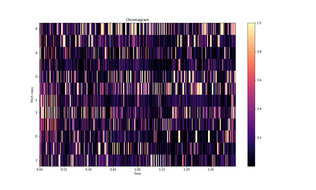
Onset Detection
Onset detection refers to a set of methods that allow us to locate the onset of notes through a sound. There are several methods to do this. They can broadly be split into the following categories:
- Energy-based methods
- Pitch-based methods
- Phase-based methods
- Supervised learning
Energy-based Methods
In energy-based methods, the spectrum is used to measure energy change in the time-frequency domain. First-order differences in spectral values have been used to find the onsets in past but are imprecise. According to psychoacoustic principles, a similar change in frequency can be detected better at lower amplitudes. A relative differencing scheme helps us find peaks better.
For example, spectrum D can be defined as follows:
$$ D_{m}(n) = 20log_{10}(|X_m(n)|^{2}) - 20log_{10}(|X_m(n-1)|^{2}) $$
where $X_{m}(n)$ is the discrete STFT of the input signal.
The commonly-used energy-based detection methods can be generalized as follows:
$$ M = \frac{1}{N} \sum_{m=1}^{N} H(D_{m}(n)) $$
Where $ H(x) = \frac{x + |x|}{2} $ is the half-wave rectifier function, N is the total number of frequency bins in the spectrum D, and M is the detection function.
The detection function is further smoothed with a moving average. A simple peak-picking operation is applied to find the onsets. Peaks with values over a certain threshold are returned as onsets.
Phase-based Methods
STFT can be considered a band-pass filter where $X_m(n)$ denotes the output of $m^{th} $ filter. In cases where there is only one stable sinusoid component passing the $m^{th} $ band-pass filter, the output of the $m^{th} $ filter must have a constant or nearly constant frequency.
Hence the difference between consecutive unwrapped phase values must remain approximately constant too.
$$ \phi_{m}(n) - \phi_{m}(n - 1) \approx \phi_{m}(n - 1) - \phi_{m}(n - 2) $$
or
$$ \bigtriangleup \phi_{m}(n) \approx \phi_{m}(n) - 2 \phi_{m}(n - 1) - \phi_{m}(n - 2) \approx 0 $$
During transitions, the frequency isn't constant. Hence the $\bigtriangleup \phi_{m}(n) $ tends to be high.
Pitch-based Methods
Pitch-based methods use pitch characteristics to segment the sound into steady state and transient parts such that onsets are found only in the transient parts.
In A Casual Rhythm Grouping, Kristoffer Jensen suggests a detection function called the perceptual spectral flux in which the difference in frequency bands is weighed by the equal-loudness contours.
Equal loudness contours or Fletcher-Munson curves are contours of sound in the frequency domain when the listener perceives a constant amplitude for steady tones of sound.
$$ PFS_{n} = \sum_{m=1}^{N}W(X_{m}(n)^{1/3} - X_{m}(n - 1)^{1/3})$$
$X_{m}$ is the magnitude of the STFT, obtained using a Hanning window. $W$ is the frequency weighting used to obtain a value closer to the human loudness contour and the power function is used to simulate the intensity-loudness power law. The power function furthermore reduces random amplitude variations.
Supervised Learning
Neural networks have been utilized to detect onset frames in an audio signal too. A typical neural network-based onset detection pipeline looks like this:
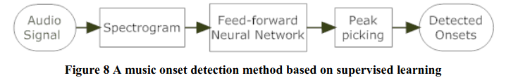
An audio signal is first converted into its spectrogram. This spectrogram is passed to a neural network that tries to classify each frame as either an onset or not. The ones that are classified as onsets are then passed through a peak-picking operation like thresholding.
There are several neural network architectures that can be utilized for this problem. The most popular choices have been recurrent networks and convolutional neural networks. Recently, audio transformers are becoming a popular choice for music classification.
The same networks can be repurposed for onset detection. Miyazaki et al, for example, use a hybrid of convolutional networks and transformer blocks for onset detection.
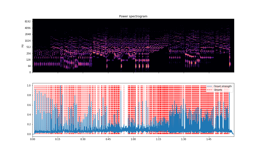
librosa has onset detection features in their API and can be used as follows.
o_env = librosa.onset.onset_strength(x, sr=sampling_rate)
times = librosa.times_like(o_env, sr=sampling_rate)
onset_frames = librosa.onset.onset_detect(onset_envelope=o_env, sr=sampling_rate)

fig, ax = plt.subplots(nrows=2, sharex=True, figsize=(15,9))
librosa.display.specshow(S_dB, x_axis='time',
                         y_axis='log', ax=ax[0])

ax[0].set(title='Power spectrogram')
ax[0].label_outer()
ax[1].plot(times, o_env, label='Onset strength')
ax[1].vlines(times[onset_frames], 0, o_env.max(),
             color='r', alpha=0.9,
             linestyle='--', label='Onsets')
ax[1].legend()

plt.savefig('onsets.png')
The visualization will be able to point out estimated locations of places where a new note is played through the audio.
A visualization of the first five seconds can be obtained like this.
o_env = librosa.onset.onset_strength(x, sr=sampling_rate)
total_time = librosa.get_duration(x)
five_sec_mark = int(o_env.shape[0]/total_time*5)
o_env = o_env[:five_sec_mark]
times = librosa.times_like(o_env, sr=sampling_rate)
onset_frames = librosa.onset.onset_detect(onset_envelope=o_env, sr=sampling_rate)

fig, ax = plt.subplots(nrows=2, sharex=True, figsize=(15,9))
librosa.display.specshow(S_dB[:, :five_sec_mark], x_axis='time',
                         y_axis='log', ax=ax[0])

ax[0].set(title='Power spectrogram')
ax[0].label_outer()
ax[1].plot(times, o_env, label='Onset strength')
ax[1].vlines(times[onset_frames], 0, o_env.max(),
             color='r', alpha=0.9,
             linestyle='--', label='Onsets')
ax[1].legend()

plt.savefig('onsets-5secs.png')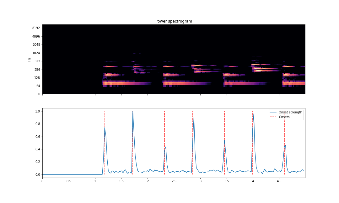
As we can see above, the vertical lines are lined up correctly where note onsets are found. The vertical lines are plotted against the magnitude curve. The spectrogram is displayed above with the same X-axis to compare note onset visually.
Beat and Tempo
A beat in music theory is a unit of time that tracks the periodic element in music. You can think of beats as the times you tap your feet while listening to a song. The tempo of a song is the number of beats per minute. The tempo might change over the course of the song.
Detecting beats and estimating the tempo of a song are closely related to onset detection. Usually, detecting beats and tempo of a song is done in three steps:
- Onset detection: computing the locations of onsets based on spectral flux
- Periodicity estimation: computing periodic patterns in the onset locations
- Beat location estimation: computing location of beats depending on the onsets and the periodicity information
In Tempo and Beat Estimation of Musical Signals, the authors give the following definition for spectral flux:
$$ E(m,n) = \sum_{n} h(n - k)G(m,n)$$
where $h(n)$ approximates a differentiator filter and
$$ G(m,n) = \mathcal{F}\{|X(m,n)|\}$$
where $X(m,n)$ is the STFT of our signal.
The transformation $\mathcal{F}$ takes the STFT of the signal and passes it through a low-pass filter and nonlinear compression algorithm using the inverse hyperbolic sine function.
The authors then use a median filter to pick out the onsets that are true note attacks instead of low-amplitude peaks.
The result of this detection function can be thought of as a pulse train which has a high magnitude at note attacks. This can be done in two ways.
Spectral Product
The idea here is that strong harmonics are found at frequencies which are an integer multiple of the fundamental frequency.
To find this frequency, we calculate the discrete Fourier transform of the signal and get a product of all of its values, leading to a reinforced frequency.
The estimated tempo T is then easily obtained by picking out the frequency index corresponding to the largest peak of the reinforced frequency values. The tempo is required to be between 60 and 200 BPM or beats per minute.
Autocorrelation
The classic approach to finding the periodicity in an audio signal is using autocorrelation. ACF or autocorrelation function can be defined as
$$r(\tau) = \sum_{k}p(k + \tau)p(k)$$
where $\tau$ is the lag value. To find the estimated tempo, the lag of the three largest peaks of $r(\tau)$ are analyzed. In the case that no multiplicity relationship is found, the lag of the largest peak is taken as the beat period.
To find the beat locations, an artificial pulse train is created of tempo T using either spectral product or autocorrelation functions. We then cross-correlate this with the original detection function output.
We call the time index where the correlation is maximum $t_{0}$ and the first beat. The second and subsequent beats in a given analysis window are found by adding a beat period $\mathcal{T}$
$$t_{i} = t_{i-1} + \mathcal{T}$$
librosa allows us to calculate a static tempo, dynamic tempo and also visualize the BPM over time using a tempogram.
To calculate the static tempo, run the following code:
onset_env = librosa.onset.onset_strength(x, sr=sampling_rate)
tempo = librosa.beat.tempo(onset_envelope=onset_env, sr=sampling_rate)
print(tempo)
You should get a single element array as the output:
array([107.66601562])To get the dynamic tempo:
dtempo = librosa.beat.tempo(onset_envelope=onset_env, sr=sampling_rate,
                            aggregate=None)
print(dtempo)
The result is an array:
array([112.34714674, 112.34714674, 112.34714674, ..., 107.66601562, 107.66601562, 107.66601562])You can also visualize the dynamic tempo using the tempogram:
fig, ax = plt.subplots(figsize=(15,9))
tg = librosa.feature.tempogram(onset_envelope=onset_env, sr=sampling_rate,
                               hop_length=hop_length)
librosa.display.specshow(tg, x_axis='time', y_axis='tempo', cmap='magma', ax=ax)
ax.plot(librosa.times_like(dtempo), dtempo,
         color='c', linewidth=1.5, label='Tempo estimate (default prior)')
ax.set(title='Dynamic tempo estimation')
ax.legend()
plt.savefig('tempogram.png')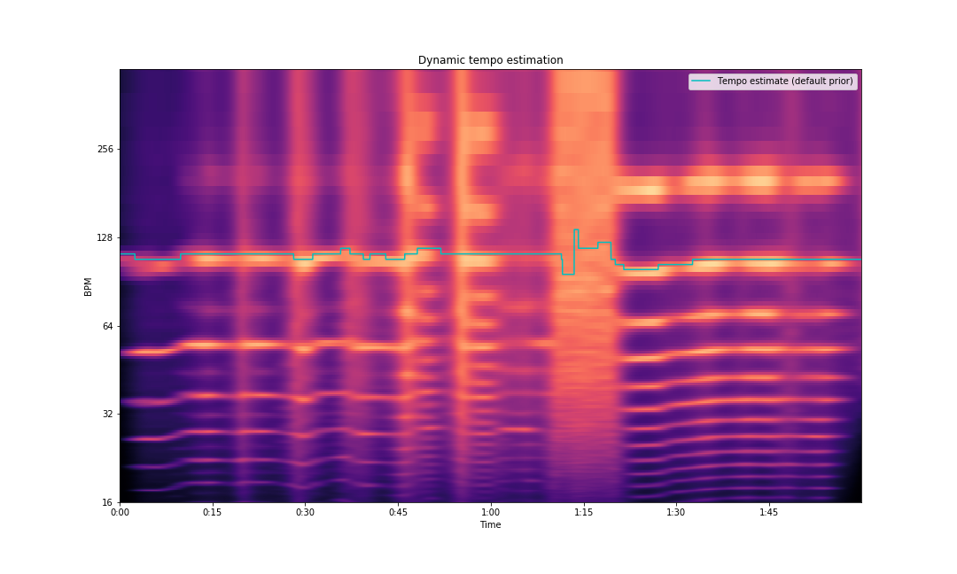
Spectrogram Decomposition
Spectrograms can provide a lot more information about a sound that just visual cues on onset and frequencies. We can use spectrograms to separate different components of a piece of music.
One of the most common use cases would be to separate harmonic sounds from the percussive sounds, e.g. piano, keyboard, guitar, and flute compared to drums, bongos, etc. This can be done using the Harmonic Percussive Source Separation algorithm or HPSS.
Harmonic Percussive Source Separation (HPSS)
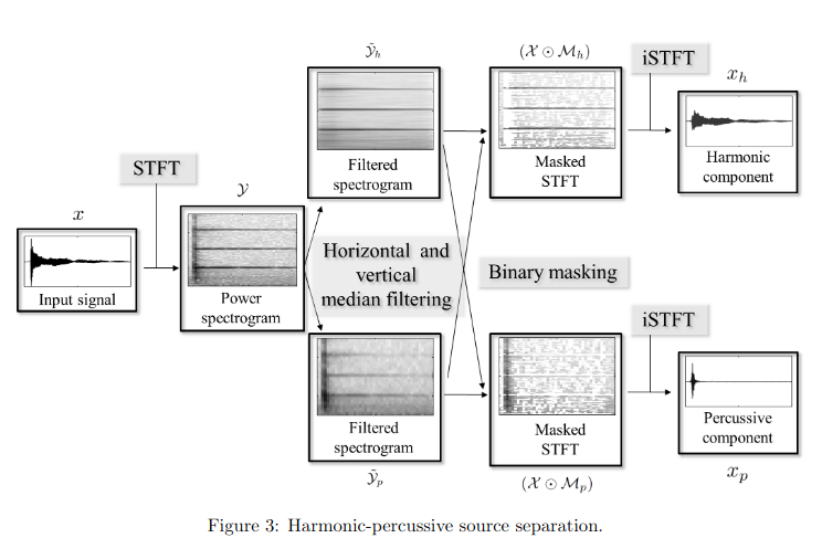
The HPSS algorithm has 4 steps to it:
- Calculating the spectrogram
- Vertical and horizontal median filtering
- Binary masking of the filtered spectrogram
- Inverting the masked spectrogram
We know that given an ordered list of $N$ values, the median is the $((N-1)/2)^{th}$ value if $N$ is odd or else the sum of the $(N/2)^{th}$ and $((N+1)/2)^{th}$ terms.
Then, given a matrix $B \in R_{N×K}$, we define harmonic and percussive median filters as follows:
$ medfilt_{h}(B)(n,k) = median({B(m−l_{h},k),...,B(m+l_{h},k)})$
$medfilt_{p}(B)(n,k) = median({B(n,k−l_{p}),...,B(n,k+l_{p})})$
where $2l_{h} + 1$ and $2l_{p} + 1$ are the length of the harmonic and percussive filters respectively. The enhanced spectrograms are them calculated as follows.
$ \phi_{h} = medfilt_{h}(|X(n, k )|^{2})$
$ \phi_{p} = medfilt_{p}(|X(n, k )|^{2})$
where $X(n,k)$ is the STFT of the sound signal.
Binary masking is applied on the filtered spectrograms. For the harmonic spectrogram, the values of the element $ M_{h}(n,k)$ is $1$ if the value of$ \phi_{h}(n,k)$ is greater than or equal to $\phi_{p}(n,k)$. Otherwise the value of $M_{h}(n,k)$ is 0.
Similarly, for the percussive spectrogram, the values of the element $ M_{p}(n,k)$ is $1$ if the value of $\phi_{p}(n,k)$ is greater than $\phi_{h}(n,k)$. Otherwise the value of $M_{p}(n,k)$ is 0.
Note that this formulation means that $M_{h}(n,k) + M_{p}(n,k) = 1$ for all $n$ and $k$. To get the spectrogram of the percussive and harmonic elements, we do an element-wise multiplication between the original STFT $X$ and the binary masks $M_{p}$ and $M_{h}$.
Due to our definition of binary masking, every frequency bin at every point is time is either assigned to $X_{h}$ or $X_{p}$.
$$ X_{h} = X \bigodot M_{h} $$
$$ X_{p} = X \bigodot M_{p} $$
Once you have these, you can get the percussive and harmonic elements of the signal by applying an inverse STFT.
librosa provides an out of the box implementation for the HPSS algorithm.
S = librosa.stft(x)
H, P = librosa.decompose.hpss(S)

fig, ax = plt.subplots(nrows=3, sharex=True, sharey=True)
img = librosa.display.specshow(librosa.amplitude_to_db(np.abs(S), ref=np.max),
                         y_axis='log', x_axis='time', ax=ax[0])
ax[0].set(title='Full power spectrogram')
ax[0].label_outer()
librosa.display.specshow(librosa.amplitude_to_db(np.abs(H), ref=np.max(np.abs(S))),
                         y_axis='log', x_axis='time', ax=ax[1])
ax[1].set(title='Harmonic power spectrogram')
ax[1].label_outer()
librosa.display.specshow(librosa.amplitude_to_db(np.abs(P), ref=np.max(np.abs(S))),
                         y_axis='log', x_axis='time', ax=ax[2])
ax[2].set(title='Percussive power spectrogram')
fig.colorbar(img, ax=ax, format='%+2.0f dB')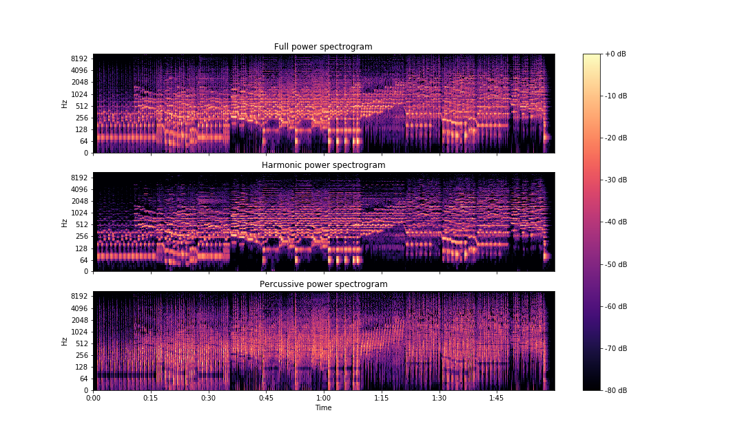
You can get the segregated signals as follows:
y_harm = librosa.istft(H)
y_perc = librosa.istft(P)
librosa implementation also allows to decompose the signal into three elements instead of two: harmonic, percussive and residual. You can do this by setting the margin argument's value as anything greater than 1.
H, P = librosa.decompose.hpss(S, margin=3.0)
R = S - (H + P)
y_harm = librosa.istft(H)
y_perc = librosa.istft(P)
y_res = librosa.istft(R)
Conclusion
In this article, we explored notes, harmonics, octaves, chroma representation, onset detection methods, beat, tempo, tempograms, and spectrogram decomposition using the HPSS algorithm.
In the next part of this series, we will try to build a text to speech engine with deep learning. As we all like to say – stay tuned!