
Bring this project to life
In this guide, we will explore mixed-precision training to understand how we can leverage it in our code, how it fits into the traditional deep learning algorithmic framework, what frameworks support mixed precision training and the performance tips of GPUs using Mixed Precision in order to look at some real world performance benchmarks.
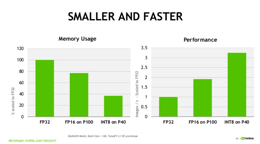
As deep learning approaches evolve, it becomes clear that increasing the size of a neural network improves performance. However, this comes at the expense of higher memory and computation needs in order to train the model. We will later look at the advantage of mixed precision training on GPU memory.
This can be viewed in context by evaluating the performance of BERT, Google's pre-trained language model, at various architectural sizes.
Last year, Google released and open-sourced Bidirectional Encoder Representations from Transformers, or BERT for short, a neural network-based approach for natural language processing (NLP). Anyone may use this technique to train their own cutting-edge question answering system to operate faster and consume less memory while maintaining model accuracy.
In 2017, a group of NVIDIA researchers published a paper describing how to minimize the memory needs of training neural networks by employing a technique known as Mixed Precision Training
This blog post will be of interest to framework developers, users who wish to optimize the advantages of their mixed-precision training, and researchers working on training numerics.
First, we will try to understand Mixed Precision Training and it's connection to deep learning, before we explore how to leverage it in our code. After that, we will explore what frameworks support mixed precision training.
What do you know about Mixed Precision Training?
Mixed precision training involves the employment of lower-precision operations (float16 and bfloat16) in a model during training to help training run quickly and consume less memory.
Using mixed precision may boost performance by more than three times on newer GPUs and by 60 percent on TPUs. Each successive generation of Nvidia GPUs, for example, has enhanced Tensor Cores and other technologies that enable better and better performance.
Notations
- FP16 — Half-Precision, 16 bit Floating Point-occupies 2 bytes of memory.
- FP32 — Single-Precision, 32 bit Floating Point-occupies 4 bytes of memory.
The basic concept of mixed precision training is straightforward: half the precision (FP32 - FP16), half the training time.
The Pascal architecture enabled the ability to train deep learning networks with reduced precision, which was originally supported in CUDA® 8 in the NVIDIA Deep Learning SDK.
The image below (source: Nvidia) shows the comparison of FP16 and other data transfer types - The FP16 is faster compared to FP32.
Most framework developers use single precision floating point numbers for all computing kernels while training deep learning models. This Paperspace blog by James Skelton, demonstrates that reduced precision training works for several models trained on limited datasets. Additionally, 16 bit half precision floating point numbers are sufficient to train large deep learning models on bigger datasets efficiently. This allows hardware sellers to make use of the available computing power.
The parameters discussed above require half of the maximum storage for the entire model. The minimum precisions required for arithmetic operations are set to 16 and 32 bits respectively. When employing 16-bit precision and maintaining some important sections of the model in float32, the model will run quicker during training as well as when using 32-bit precision.
Recent versions of NVIDIA GPUs include particularly unique tensor cores developed specifically for rapid FP16 matrix computations. But, until relatively recently, these Tensor Cores have been challenging to employ since they required hand-written decreased precision computations into your model.
Automatic Mixed Precision Training with Deep Learning
Deep neural networks (DNNs) have transformed artificial intelligence by achieving exceptional accomplishment in intelligence tests such as image and speech recognition. However, training big DNNs is computationally costly, which has driven the quest for innovative hardware platforms aimed towards this function.
As a result, a mixed-precision training architecture is often used, which combines a computational memory unit that performs weighted summaries and inaccurate conductance updates with a digital processing unit that gathers weight updates with high accuracy.
A mixed software training experiment of a recurrent neural network evaluation of the proposed architecture using a phase-change memory (PCM) array achieves 97.73 percent test accuracy on the task of classifying handwritten digits (based on the MNIST dataset), within 0.6 percent of the software reference point.
The design is then tested on a variety of networks, including convolutional neural networks, long-short-term memory networks, and generative-adversarial networks, utilizing correct appropriate models of PCM.
Accuracy equivalent to floating-point implementations is attained without being bound by the non-idealities of PCM devices. When used to train a multilayer perceptron, the architecture's energy efficiency improves by 172 when compared to a completely dedicated digital 32-bit implementation, according to a system-level research.
Due to increased computing and data transport throughputs, mixed precision has become the standard arithmetic for speeding deep learning models. Deep learning models, which are frequently trained using IEEE single-precision formats, are found to be resilient to representation length reduction when utilizing mixed precision, since they can match state-of-the-art performance. To avoid gradient underflow, the user may either fix the value of their loss scaling or utilize the automated loss scaling strategy, which will algorithmically decide the appropriate value of scaling to apply.
Code Walkthrough with PyTorch
With that critical previous knowledge out of the way, we can safely dive into the new PyTorch AMP API.
This section contains simple walkthrough of how to code a convolutional neural network (CNN) using the PyTorch library for mixed precision training.
For demonstration, we will train it on the very common MNIST dataset of handwritten digits.
With this code, we go through how to create the network as well as initialize a loss function, optimizer, check accuracy and more.
Before getting started, make sure Python3 is installed on your machine.
Let’s create a workspace for this project and install the dependencies you’ll need using the Terminal.
You can skip steps 1-5 and jump right into the demo by clicking the Run On Gradient button linked below!
Bring this project to life
- Name your workspace py-torch:
$ mkdir ~/pytorch2. Create a folder to keep your assets:
$ mkdir ~/pytorch/assets3. Navigate to the pytorch directory
$ cd ~/pytorch4. Create a new virtual environment for the project
$ python3 -m venv pytorch5. Activate your environment
$ source pytorch/bin/activate6. Install PyTorch
pip install torch==1.7.1+cpu torchvision==0.8.2+cpu -f https://download.pytorch.org/whl/torch_stable.html7. To make this section a little fast track, edit the imports in your py-torch.py file to look exactly like this:
#Imports
import torch
import torchvision # torch package for vision related things
import torch.nn.functional as F  # Parameterless functions, like (some) activation functions
import torchvision.datasets as datasets  # Standard datasets
import torchvision.transforms as transforms  # Transformations we can perform on our dataset for augmentation
from torch import optim  # For optimizers like SGD, Adam, etc.
from torch import nn  # All neural network modules
from torch.utils.data import DataLoader  # Gives easier dataset managment by creating mini batches etc.
from tqdm import tqdm  # For nice progress bar!
Next: Check out my code on this repository here and copy into your py-torch.py workspace:
8. Edit the Simple CNN section, by increasing the out-channels in line 18 of our code to 420, in_channels = 420, out_channels = 1000, and nn.Linear to 1000. Use the code snippet below line by line.
# Simple CNN
class CNN(nn.Module):
    def __init__(self, in_channels=1, num_classes=10):
        super(CNN, self).__init__()
        self.conv1 = nn.Conv2d(
            in_channels=in_channels,
            out_channels=420,
            kernel_size=(3, 3),
            stride=(1, 1),
            padding=(1, 1),
        )
        self.pool = nn.MaxPool2d(kernel_size=(2, 2), stride=(2, 2))
        self.conv2 = nn.Conv2d(
            in_channels=420,
            out_channels=1000,
            kernel_size=(3, 3),
            stride=(1, 1),
            padding=(1, 1),
        )
        self.fc1 = nn.Linear(1000 * 7 * 7, num_classes)
9. Here, let us define another function under the CNN class with two parameters that returns the value of our computation:
You can follow through my code to ensure you don't miss out.
def forward(self, x):
        x = F.relu(self.conv1(x))
        x = self.pool(x)
        x = F.relu(self.conv2(x))
        x = self.pool(x)
        x = x.reshape(x.shape[0], -1)
        x = self.fc1(x)
        return x
10. Setup the device
device = torch.device("cuda" if torch.cuda.is_available() else "cpu")11. Configure the hyperparameters
Ensure that the limit is at a batch_size of 590 for a float32 or 1000 for a float16. However, we should always use float16 as default when training networks.
in_channels = 1
num_classes = 10
learning_rate = 0.001
batch_size = 590
num_epochs = 3
12. Next we load in our data:
train_dataset = datasets.MNIST(root="dataset/", train=True, transform=transforms.ToTensor(), download=True)
test_dataset = datasets.MNIST(root="dataset/", train=False, transform=transforms.ToTensor(), download=True)
train_loader = DataLoader(dataset=train_dataset, batch_size=batch_size, shuffle=True)
test_loader = DataLoader(dataset=test_dataset, batch_size=batch_size, shuffle=True)
13. Initialize the neural network
model = CNN(in_channels=in_channels, num_classes=num_classes).to(device)14. Loss and Optimizer: here we setup the float16 training to see how much of a larger batch size we can now use before our training loop.
criterion = nn.CrossEntropyLoss()
optimizer = optim.Adam(model.parameters(), lr=learning_rate)
scaler = torch.cuda.amp.GradScaler()
15. Executing a custom training loop with mixed precision needs two modifications as opposed to walking it in float32;
# Train Network
for epoch in range(num_epochs):
    for batch_idx, (data, targets) in enumerate(tqdm(train_loader)):
        # Get data to cuda if possible
        data = data.to(device=device)
        targets = targets.to(device=device)

        # forward
        with torch.cuda.amp.autocast():
        	scores = model(data)
        	loss = criterion(scores, targets)

        # backward
        optimizer.zero_grad()
        scaler.scale(loss).backward()
        scaler.step(optimizer)
        scaler.update()
16. Define a function to check accuracy on training ;
def check_accuracy(loader, model):
    num_correct = 0
    num_samples = 0
    model.eval()

    with torch.no_grad():
        for x, y in loader:
            x = x.to(device=device)
            y = y.to(device=device)

            scores = model(x)
            _, predictions = scores.max(1)
            num_correct += (predictions == y).sum()
            num_samples += predictions.size(0)


    model.train()
    return num_correct/num_samples
Final Step: Test our code to see how good our model is:
print(f"Accuracy on training set: {check_accuracy(train_loader, model)*100:.2f}")
print(f"Accuracy on test set: {check_accuracy(test_loader, model)*100:.2f}")
You can also check out more information on Mixed-Precision training in NVIDIA official documentation.
Mixed Precision Training Deep Learning Frameworks
TensorFlow, PyTorch, and MXNet are the frameworks that currently offer automated mixed precision.
For all the frameworks, using Mixed Precision will require three major steps;
- Converting the model to use the float16 data type where possible.
- Keeping float32 master weights to accumulate per-iteration weight updates.
- Using loss scaling to preserve small gradient values.
For the rest of this article, we will focus on TensorFlow as it is commonly used with Paperspace GPUs from the Maxwell, Pascal, Volta, Turing, and Ampere microarchitectures.
Enabling Mixed Precision Training in Tensorflow
In TensorFlow, Mixed Precision can be enabled using the Automatic Mixed Precision extension (TF-AMP) which models variables to half-precision upon recapture, while keeping variables in single precision format.
Moreover, when using gradients, a loss amplification step must be incorporated to protect tiny gradient magnitudes in stochastic gradient descent. Loss scaling in TensorFlow may be done statically by multiplying the loss by a fixed amount or automatically, by TF-AMP. Automatic mixed precision does all changes within TensorFlow, giving two advantages over manual processing.
First, developers do not need to adjust network model code, which reduces development and maintenance time. Furthermore, leveraging AMP ensures forward and backward compatibility with all TensorFlow APIs for defining and executing models.
Purely add the values to the environmental variables within your training script to allow mixed precision:
- Enable TF-AMP graph rewrite:
os.environ["TF_ENABLE_AUTO_MIXED_PRECISION_GRAPH_REWRITE"] = "1"- Enable Automated Mixed Precision:
os.environ['TF_ENABLE_AUTO_MIXED_PRECISION'] = '1'
Enabling TensorFloat-32
Tensor operations are the new math mode in Nvidia A100 GPUs for computing matrix math using the TF32. They can provide up to 10 times speedups compared to single-precision floating-point math (FP32) on Volta GPUs.
TF32 Tensor Cores can speed up networks using FP32, typically with no loss of accuracy. It is more robust than FP16 for models which require high dynamic range for weights or activations.
TF32 is supported in the NVIDIA Ampere GPU architecture and is enabled by default.
More details may be found in the TensorFloat-32 section of the A100 GPU Accelerates AI Training, HPC Up to 20x blog article. You can also see how the A100 stacks up to Paperspace's diverse GPU selection by going to the GPU Cloud Comparison.
Understanding the TensorFloat-32 Math
Math formats are similar to rulers. The amount of bits in the modulus of a format affects its scope, or the size of the item it can evaluate. The precision is determined by the amount of bits utilized by its mantissa, the component of its floating point number following the radix or decimal point.
A great math format fits in the perfect balance. To provide precision, it should utilize sufficient bits to avoid slow performance or memory bloating.
The plot below from Nvidia depicts how TF32 is a blend that achieves this balance for tensor computations.
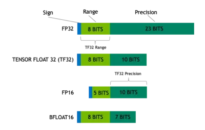
TF32 employs the same 10-bit mantissa as half-precision (FP16) math, which has been proven to provide more than enough tolerance for the precision standards of AI tasks. TF32 also uses the same 8-bit multiplier as FP32, allowing it to handle the same mathematical limit.
Because of this, TF32 is an amazing addition to FP32 for doing single-precision math, particularly the huge multiply-accumulate operations at the core of deep learning and several HPC applications.
Applications that use NVIDIA libraries allow users to reap the benefits of TF32 with no code changes. TF32 Tensor Cores process FP32 inputs and output FP32 results. FP32 is still used for non-matrix computations. The A100 also features increased 16-bit math capability for optimal performance. It supports FP16 and Bfloat16 (BF16) at double the speed of TF32. With just a few lines of code, users may get a 2x increase in speed by using Automated Mixed Precision.
Successful TensorFlow Projects
This section discusses a script and recipe used to train the BERT model for TensorFlow used to achieve state-of-the-art accuracy which is tested and maintained by NVIDIA. Check out the public repository for this model here.
This repository contains scripts to interactively launch data download, training, benchmarking and inference routines in a Docker container for both pre-training and fine tuning for Question Answering.
BERT Model Overview
The BERT (Bidirectional Encoder Representations from Transformers) used by NVIDIA, is a customized replica of Google's official implementation, and uses mixed precision arithmetic and Tensor Cores on A100, V100 and T4 GPUs for faster training speed while maintaining precision.
You can check out this public repository that provides the BERT model by NVIDIA. It is trained with mixed precision using Tensor Cores on NVIDIA Volta, Ampere and Turing GPUs. This means, programmers can get responses up to 4x faster than training without Tensor Cores, while experiencing the advantages of mixed precision training.
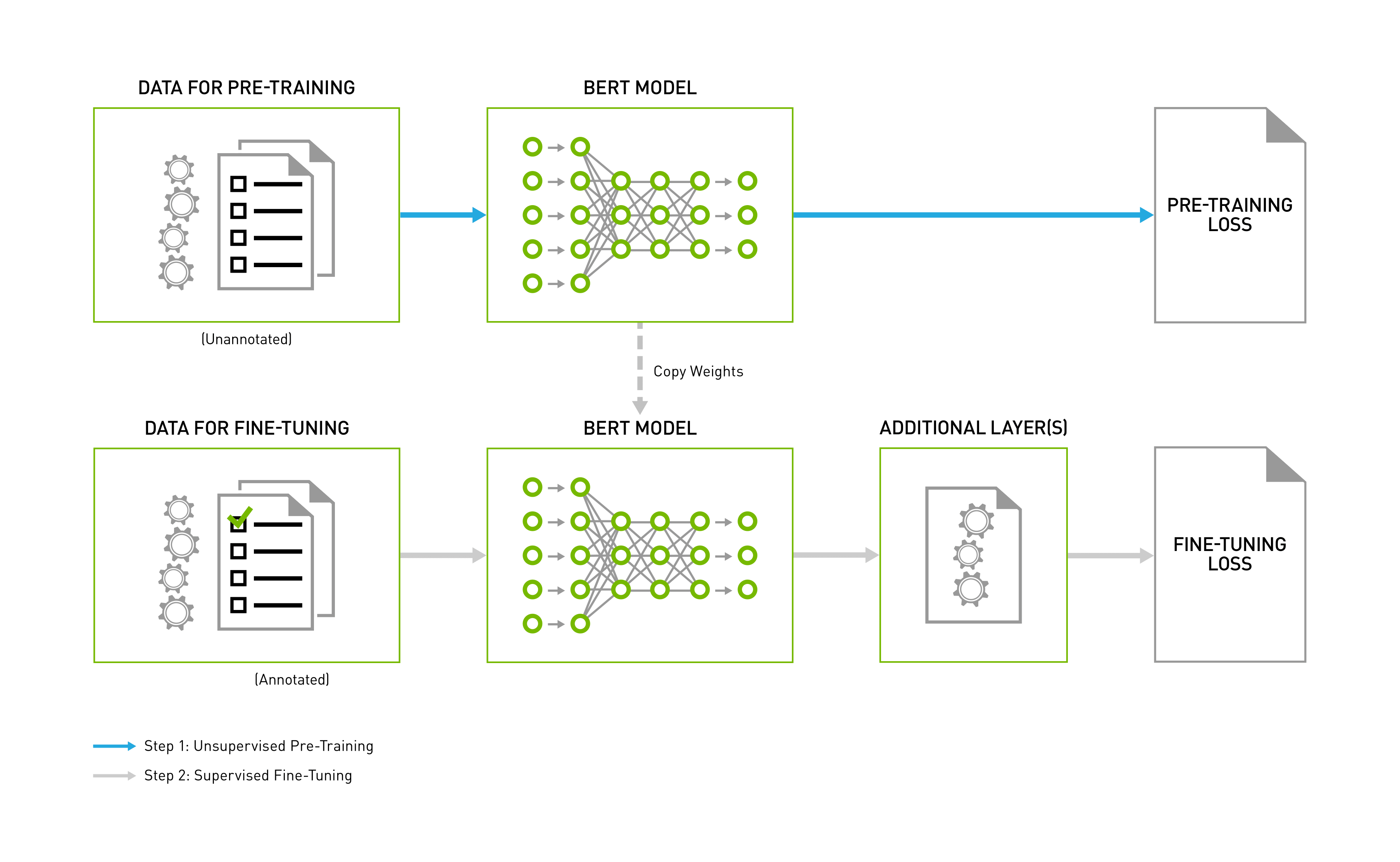
Architecture of the BERT model
The architecture of the BERT model is a complex bidirectional Transformer encoder. According to the model size, the BERT training consists of two steps, which pre-trains the language model in an unsupervised fashion on vast amounts of unannotated datasets, and also using this pre-trained model for fine-tuning in numerous NLP activities. This model provides an additional layer for the precise task and further trains the model to use a task-specific annotated dataset, beginning with pre-trained weights. The initial and final stages of the process are as shown in the image below;
Performance tips when using mixed precision on GPUs.
Increasing batch size
If it has no effect on model quality, try running with double the batch size while using mixed precision. Because float16 tensors utilize half the capacity, you may frequently double your batch size without running out of memory. Boosting batch size often increases training throughput, or the number of training components your model can run on per session.
Ensure the utilization of GPU Tensor Cores
Modern NVIDIA GPUs include a specific hardware unit known as Tensor Cores, which can rapidly multiply float16 matrices. Tensor Cores, on the other hand, mandates that certain tensor dimensions be a multiple of 8.
If you want to learn further, the NVIDIA deep learning performance guide provides the specific requirements for using Tensor Cores as well as increased performance statistics relating to Tensor Cores.
Real World Performance benchmarks
The Spell API is used to train neural networks with automatic precision and also using the V100s (older tensor cores) and T4s (present tensor cores). Each of the mentioned models converge equally when used between the mixed precision and vanilla network. Here is a list of networks trained with the mentioned models:
- Feedforward - a neural network trained on data obtained from Rossman Store Samples competition on Kaggle. Browse the code here.
- UNet - a vanilla UNet picture segmentation net of medium size trained on the Segmented Bob Ross Images corpus. Get the code by clicking here.
- BERT - an enormous NLP transformer model built with huggingface's bert-base-uncased model backbone and data from Kaggle's Twitter Sentiment Extraction competition. Get the code by clicking here.
Sample Results:
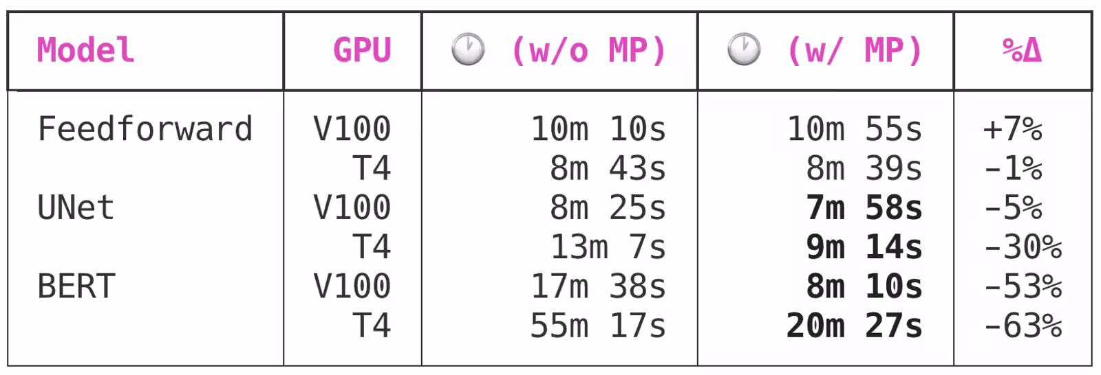
BERT is a huge model, and it is here that the time savings of adopting mixed precision training become "must-have." Automatic mixed precision will save time training by 50 to 60% for big models trained on Volta or Turing GPUs.
Therefore, one of the first performance improvements you should apply to your model training scripts is mixed precision.
If you want to replicate any benchmarks yourself, example model source code is available on GitHub in the spellrun/feedforward-rossman, spellrun/unet-bob-ross, and spellrun/tweet-sentiment-extraction repositories.
To run these with Paperspace Gradient, simply use the previous URL's as the Workspace URL in the advanced options section of the Notebook create page.
GPU Memory Bandwidth Usage
Now that we understand how mixed precision works from our previous sections. One advantage of mixed precision training is memory usage. GPU compute is more complex compared to GPU memory, however it is important to optimize. Remember, the greater the batch sizes you can put on the GPU, the more efficient your memory consumption.
PyTorch allocates a fixed amount of GPU memory at the start of the model training process and keeps it for the life of the training operation. This prevents other tasks from committing too much GPU RAM during training, which would otherwise cause the PyTorch training script to crash with an OOM error.
The following is the effect of activating mixed precision training on PyTorch memory reservation behavior:
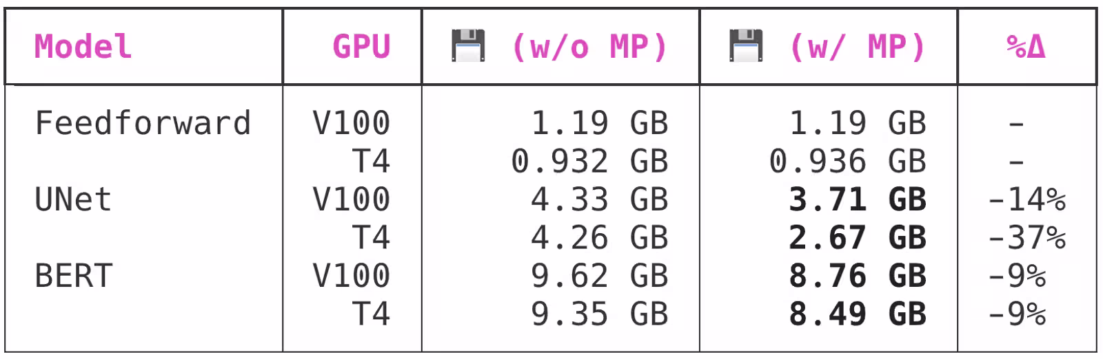
Surprisingly, while both of the bigger models profited from the switch to mixed precision, UNet benefited far more than BERT.
Takeaways
Automatic mixed precision training is a simple and powerful new feature in PyTorch 1.6 that promises to speed up larger-scale model training operations running on modern NVIDIA GPUs by up to 60%.
As detailed in this article, technological advancement from generation to generation of GPU can be partially characterized by Mixed Precision Training and therefore should be implemented wherever possible. Paperspace are here to help optimize your GPU cloud spend and efficiency if you are in need.
Additionally, when utilizing an RTX, Tesla, or Ampere GPU, Gradient users should employ automated mixed precision training. These GPUs include Tensor Cores, which speed up FP16 operations.


