Mixed Precision Training

Introduction

A computing approach that uses a combination of multiple numerical precisions is known as mixed precision. Mixed-precision training refers to a deep neural network training technique that employs half-precision whenever feasible and complete precision when it is not. There are two stages to using mixed-precision training:

• Porting the model to use the FP16 data type where appropriate.
• Adding loss scaling to preserve small gradient values.

This article provide a friendly overview of mixed precision training.

Some Benefits of Using Mixed Precision Training

It is possible to get up to a three-fold increase in speed by using mixed-precision training for arithmetically intensive model architectures. The benefits of employing half-precision in memory-constrained systems may also lead to a boost in performance. Training deep neural networks with a precision lower than 32-bit floating point has several advantages.

Lower precision needs less memory to train more extensive networks. As a result, the training process is more efficient since it takes less memory bandwidth. Finally, the lower the precision, the speedier the mathematical operations may be carried out.

What Does It Mean When We Talk About "Lower Precision"?

The 32-bit floating-point (FP32) format is referred to as single precision. When we say "lower precision," we generally refer to the 16-bit floating-point (FP16) format.
As their names imply, the FP32 format uses 32 bits of memory, whereas the FP16 format uses 16 bits of memory.

Consequently, the number of bytes accessed is also reduced. Going from FP32 to FP16, on the other hand, lowers precision, which is essential when working with tiny activation gradient values in deep learning. FP16 training accuracy suffers when gradient values are too tiny to be represented by an FP32 number but are too large to be represented by an FP16 number (in which case it becomes zero).

Gradient values can be scaled such that they fall inside FP16's range of representable values, reducing the loss of accuracy that occurs.

FP32 Master Copy of Weights: Illustration From The Paper

In mixed-precision training, weights, activations, and gradients are stored as FP16. To match the accuracy of the FP32 networks, an FP32 master copy of weights is maintained and updated with the weight gradient during the optimizer step. In each iteration, an FP16 copy of the master weights is used in the forward and backward pass, halving the storage and bandwidth needed by FP32 training.

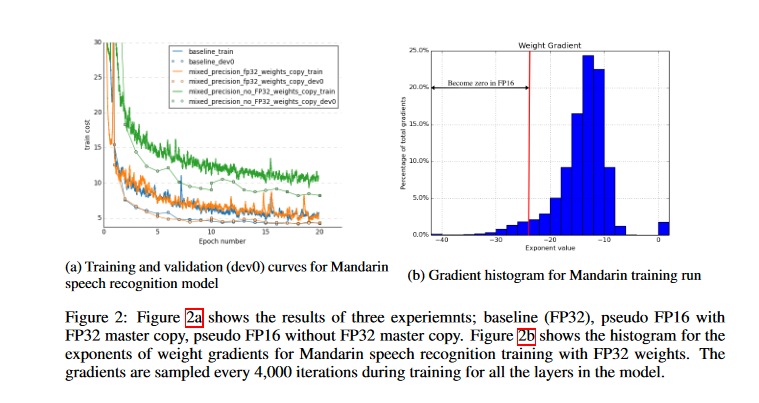
Researchers used a Mandarin speech model trained on a dataset of 800 hours of speech data for 20 epochs to demonstrate the necessity of an FP32 master copy of weights.

As seen in the graph below, updating an FP32 master copy of weights after FP16 forward and backward passes results in a match to FP32 training results; however, updating FP16 weights leads to a loss of relative accuracy of 80%. Even keeping an extra copy of weights increases weight memory needs by 50% compared to single precision training; the effect on total memory consumption is substantially lower. Because of increased batch sizes and activations of each layer being saved for reuse in the back-propagation stage, activations dominate training memory usage.

Because activations are also recorded in half-precision format, the total memory usage for deep neural network training is about halved.

Using Scaling to Prevent Loss of Accuracy

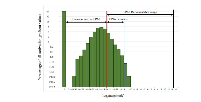
The paper highlights the fact that, while gradient values tend to be dominated by small magnitudes, the FP16 exponent bias centers the range of normalized value exponents to [−14, 15]. By taking an example from the histogram of activation gradient values gathered across all layers during FP32 training for the Multibox SSD detector network, we can observe that a large portion of the FP16 representable range was unused.

Many values fell below the minimum representable range and became zeros. It is possible to preserve values that would have otherwise been lost to zero by scaling up the gradient. Scaling up the gradients will also shift them to occupy more of the representable range.

When gradients aren't scaled, this network diverges, but scaling them by a factor of 8 is enough to achieve the same level of accuracy with FP32 training. This suggests that activation gradient values below 2^-27 in magnitude were irrelevant to the training of this model, but values in the [2^-27, 2^-24] range were essential to preserve.

A number that is too tiny to be represented in FP16 (and hence problematically represented as zero) can be retrieved by scaling it by a factor that allows for its representation in FP16. Activation gradients are the small values of interest in deep learning applications. Scaling usually occurs between the steps of forward propagation and back-propagation.

If the back-propagation input is scaled by a certain factor, then all of the subsequent activation gradients will be scaled by that factor as well; hence the remainder of the back-propagation technique does not need to be scaled.
To update the weights, the optimizer can be provided with the unscaled gradients when back-propagation is complete. Generally, the method is as follows:

• Perform forward propagation
• Scale up the output by a factor X
• Back-propagation technique application
• Scale the weight gradients down by a ratio of 1/X
• Optimizer updates weights

Choose the Scaling Factor

The loss scaling factor can be selected from various alternatives, and constant scaling is the simplest option.

From 8 to 32K, they trained a wide range of networks (many networks did not require a scaling factor). Scaling factors can be selected experimentally, or, if gradient statistics are available, a constant scaling factor can be determined directly by choosing a factor whose product has a maximum absolute gradient value less than 65,504.

Choosing a significant scaling factor has no negative as long as it does not produce overflow through back-propagation. Overflows will lead to infinities and NaNs in the weight gradients, which will permanently destroy the weights after an update. It should be noted that checking the computed weight gradients is an effective way to discover overflows.

It is more reliable to dynamically choose the loss scaling factor. It is essential to start with a significant scaling factor and reevaluate it once each training iteration is completed. It is possible to increase the scaling factor if no overflow occurs after N iterations. The weight update should be skipped if there is an overflow. The dynamic loss-scaling approach leads to the following high-level training procedure:

1. Maintain a copy of weights in FP32 as the primary copy.
2. Set S to a considerable value.
3. For each iteration:

      a. Make an FP16 copy of the weights.

       b. Forward propagation (FP16 weights and activations).

        c. Perform multiplication of the resulting loss with the scaling factor S.

        d.  Perform backward propagation (FP16 weights, activations, and their gradients).

        e. If there is an Inf or NaN in weight gradients:

              i. Reduce S.

              ii. Move on to the next iteration without updating weight.

          f.  Perform weight gradient multiplication with 1/S.

          g. Complete the weight update (including gradient clipping, etc.).

          h. S should be increased if an Inf or NaN hasn't occurred in the last N iterations.

How Tensor Cores Work

Tensor cores were launched in late 2017 in the Volta architecture, improved in the previous-generation Turing architecture, and have been refined further in the Ampere architecture. Check out the Ampere, Volta, and Turing GPUs performance values in comparison to one another on the Paperspace GPU Cloud Comparison.

Because they may outperform the standard GPU cores, Tensor Cores are a desirable feature. Nvidia Volta GPUs Tesla V100, Quadro V100, and Titan V have 640 tensor cores and can provide up to ∼TFLOPS in mixed FP16-FP32 precision.
Traditional CUDA cores, which are 5120 in total for the GPUs already stated, can provide up to ∼15 TFLOPS of performance in FP32 precision and roughly ∼7 TFLOPS of performance in FP64 precision. Indeed, the speed of tensor cores makes it feasible to investigate new applications that might benefit from this new technology.

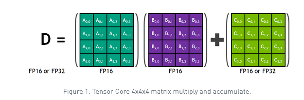
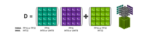
With that said, utilizing tensor cores is not without restrictions and potential pitfalls. The first restriction is that tensor core programming is substantially more restricted than typical GPU programming. If you use Tensor Cores, you can only perform MMA (matrix-multiply-accumulate) operations on 4×4 matrices (it requires just one GPU cycle), which is the only operation that can be completed when using tensor cores.

As a result, the only way to create an algorithm that can benefit from Tensor Core acceleration is to restructure it as a collection of multiple 4×4×4 MMA operations that can run in parallel.

The numerical precision is the second restriction of tensor cores. A×B+C operations are presently done in FP16 precision, even though the D matrix is stored in FP32. This hybrid manner of functioning might have detrimental implications for some applications.

Nevertheless, FP16 is an excellent place to run Tensor Cores since deep learning applications generally don't suffer from numerical precision issues during training and inference in FP16.

This operation may be a building component for more extensive FP16 matrix multiplication operations. Given that most back-propagation involves matrix multiplication, the Tensor Core may be used for any network layer requiring significant computing.

Input matrices must be in FP16 format. Your GPU isn't getting the most out of it if you're training on a tensor core-based GPU, and not utilizing mixed-precision training. You can look at this article which will give you an overview of Tensor Cores and help you understand how they work.

Tensor Cores in CUDA Libraries

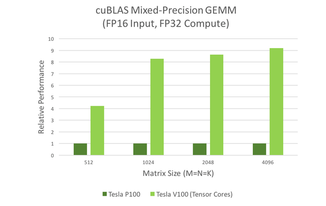
CuBLAS and cuDNN are two CUDA libraries that make use of Tensor Cores. To speed up GEMM computations, cuBLAS uses Tensor Cores. Recurrent neural networks (RNNs) and convolutions can be processed more quickly using Tensor Cores thanks to cuDNN.

GEMM is the BLAS term for matrix-matrix multiplication.

These models are widely used in signal processing, fluid dynamics, and many other fields. These applications need ever-increasing processing speeds to keep up with the ever-increasing data volumes. We can see this easily by looking at the mixed-precision GEMM performance graph in the figure below.

Neural nets are becoming more complex each year as artificial intelligence researchers push the boundaries of what is possible. The deepest networks currently exceed dozens of convolutional layers. During forward- and back-propagation, convolution layers are required to train DNNs. The figure below depicts the convolution performance chart, demonstrating that Tensor Cores can meet the need for high convolution speed.

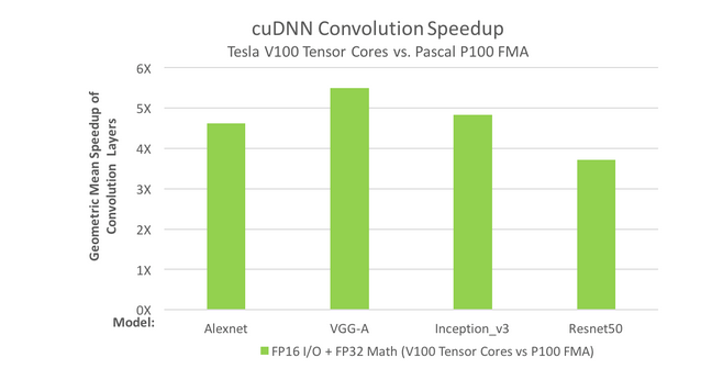
In both graphs, it can be shown that Tesla V100's Tensor Cores outperform Tesla P100's. How computing is done is changed by these kinds of gains in performance: interactive scenarios may be explored, and server farms can be used more sparingly because of these gains in performance.

Optimizing For Tensor Cores

Hardware acceleration for mixed-precision training is provided by NVIDIA Tensor Cores. It is possible to get up to an eightfold increase in float16 matrix multiply performance over float32 on a V100 GPU using Tensor Cores. Tensor Cores may need modifications to the model code to take full benefit of them. The documentation from Nvidia provides three steps to get the most out of Tensor Cores:

1. Satisfy Tensor Core shape constraints
2. Increase arithmetic intensity
3. Decrease fraction of work in non-Tensor Core operations

This list of advantages is presented in increasing complexity, with the initial stage often providing the most value for the least amount of work.

Satisfying Tensor Core Shape Constraints

Tensor Cores' inputs are constrained in shape by their architecture.
To multiply matrices, consider the following rules:

• All three dimensions in the FP16 input (M, N, and K) must be multiples of 8.
• All three dimensions must be multiples of 16 for INT8 inputs (Turing only).

When it comes to the convolution process:

• Input and output channels for FP16 inputs must be multiples of 8.
• Input and output channels on INT8 (Turing only) inputs must be multiples of 16.

An in-depth look at Tensor Core execution, where these constraints originate from, and how they materialize in real-world model designs are provided by the Deep Learning Performance Guide. The following are the recommendations from Nvidia documentation for mixed-precision training:

• Mini-batch should be a multiple of 8.
• A multiple of 8 should be chosen for the linear layer dimensions.
• Use a multiple of 8 for convolution layer channel counts.
• Pad vocabulary that is a multiple of 8 for challenges involving classification.
• Pad the sequence length multiple of 8 to solve sequence issues.

Increasing Arithmetic Intensity

Arithmetic intensity measures how much computational work will be performed in a kernel per input byte. For example, a V100 GPU has 125 TFLOPs of math throughput and 900 GB/s of memory bandwidth. Taking the ratio of the two, we see that any kernel with fewer than ~140 FLOPs per input byte will be memory-bound. Tensor Cores cannot run at full throughput because memory bandwidth will be the limiting factor. A kernel with sufficient arithmetic intensity to allow full Tensor Core throughput is compute-bound.

The arithmetic intensity can increase in both model implementation and model architecture. To increase arithmetic intensity in model implementation:

• In recurrent cells, concatenate weights and gate activations
• Sequence models allow you to concatenate activations throughout time

As a means of increasing the model's arithmetic intensity:

• Dense math operations are preferred: it is well known that depth-wise separable convolutions have lower arithmetic intensity than vanilla convolutions
• When it comes to precision, go for the widest possible layer

Decreasing Non-Tensor Core Work

Tensor Cores do not accelerate many other operations in deep neural networks, and it is critical to understand their impact on overall speedups.

Consider a model where half of its training time is spent in Tensor Core-accelerated operations. If Tensor Cores speed up those operations by 5x, the overall speedup is $1. / (0.5 + (0.5 / 5.)) = 1.67x$

Because Tensor Core operations account for a smaller and less percentage of the overall effort, optimizing non-Tensor Core processes becomes more critical. Custom CUDA implementations and framework integration can be used to speed up these processes. Compiler tools can speed up automatically non-Tensor Core operations.

Key points to remember

Using Deep Neural Networks (DNNs) has allowed significant advancements in various fields. As DNN complexity has risen to attain these achievements, researchers and users are requiring more and more computer resources to train. Using lower-precision arithmetic in mixed-precision training reduces the amount of resources needed, which has the following advantages:

• Reduce the amount of memory that is required: Single precision (FP32) uses 32 bits, whereas half-precision (FP16) uses 16 bits (FP16). Memory requirements can be reduced so that more extensive models can be trained or larger mini-batches can be trained.
• Reduce the duration of training or inferences: Memory or arithmetic bandwidth can affect execution time. Half-precision reduces the amount of time spent in memory-limited layers by halving the number of bytes accessed.

The documentation highlights three methods for training DNNs with half-precision successfully:

Accumulation into FP32

• Tensor Core instructions introduced in the NVIDIA Volta GPU architecture multiply half-precision matrices, aggregating the result into either a single- or half-precision output
• To get effective training outcomes, accumulation into single precision is essential. Before being written to memory, accumulated values are converted to half-precision

Loss Scaling

• Activations, activation gradients, weights, and weight gradients are the four kinds of tensors encountered while training DNNs
• Activations, weights, and weight gradients fall within the range of magnitudes that can be represented with a half-precision. Small-magnitude activation gradients fall below the half-precision range for certain networks
• The technique to guarantee that gradients fall within the range that can be represented by half precision is to multiply the training loss by the scaling factor
• The chain rule assures that all gradients are scaled up at no extra cost by adding a single multiplication
• Gradient values that have been lost to zero can be restored via loss scaling. Prior to the weight update, weight gradients must be scaled-down by the same factor S

The scale-down operation could be fused with the weight update itself or carried out separately.

FP32 master copy of weights

• The network weights are updated with each iteration of DNN training by adding appropriate weight gradients
• Weight gradient magnitudes are sometimes substantially less than corresponding weights, particularly when multiplied by the learning rate
• An update may not occur if one of the addends is sufficiently tiny in half-precision representation to make a significant difference
• Maintaining and updating a master copy of weights with single precision is a straightforward fix for networks that lose updates in this manner

In each iteration a half-precision copy of the master weights is made and used in both the forward- and back-propagation, reaping the performance benefits.

• The weight gradients computed during weight update are converted to single-precision and utilized to update the master copy, and the procedure is repeated in the following iteration. Consequently, we only blend half-precision and single-precision storage when necessary

Automatic Mixed Precision: NVIDIA Tensor Core Architecture in TensorFlow

NVIDIA unveiled at the 2019 GTC the Automatic Mixed Precision (AMP) functionality, which allows for automatic mixed-precision training. Using automatic mixed-precision can boost performance, but it depends on the model's architecture. Setting an environment variable or making a few code changes is all it takes to enable automated mixed precision in current TensorFlow training scripts.

With half-precision floating-point, mixed-precision training is faster while maintaining the same level of precision as single-precision training with the same hyper parameters.. As seen below, Tensor Cores, introduced in NVIDIA Volta and Turing GPU architectures, can be used with half-precision.

Although mixed-precision is possible with vanilla TensorFlow, it requires developers to make manual tweaks to the model and optimizer. Using TensorFlow's automatic mixed-precision provides two advantages over manual processes. First, the development and maintenance workload is reduced since network model code does not need to be modified by programmers. Second, AMP ensures forward and backward compatibility with all TensorFlow model definition and execution APIs.

The NVIDIA NGC TensorFlow 19.03 container (and each release since) has an automatic mixed-precision capability. To use this functionality, you just need to set one environment variable:

export TF_ENABLE_AUTO_MIXED_PRECISION=1

Alternatively, the environment variable can be specified in the Python script of TensorFlow:

os.environ['TF_ENABLE_AUTO_MIXED_PRECISION']='1'

There is a possibility to further speedups by enabling the TensorFlow XLA compiler and increasing the minibatch size.

Conclusion

In this article, we have :

• Taken a closer look at mixed-precision training as a technique.
• Seen how to use scaling to prevent loss of accuracy.
• Introduced what is tensor cores: What they are, how they work, how to optimize them.
• Seen how to use Automatic Mixed Precision for NVIDIA Tensor Core Architecture in TensorFlow

References

https://developer.nvidia.com/blog/programming-tensor-cores-cuda-9/ https://arxiv.org/abs/1903.03640
https://developer.nvidia.com/blog/mixed-precision-training-deep-neural-networks/
https://developer.nvidia.com/blog/nvidia-automatic-mixed-precision-tensorflow/
http://alexminnaar.com/2020/05/02/dl-gpu-perf-mixed-precision-training.html https://spell.ml/blog/mixed-precision-training-with-pytorch-Xuk7YBEAACAASJam; https://arxiv.org/pdf/1710.03740.pdf
https://arxiv.org/pdf/1710.03740.pdf
https://docs.nvidia.com/deeplearning/performance/mixed-precision-training/index.html#tensor-core-shape