Evaluation Metrics for Machine Learning Models: Part 1

If training models is one significant aspect of machine learning, evaluating them is another. Evaluation measures how well the model fares in the presence of unseen data. It is one of the crucial metrics to determine if a model could be deemed satisfactory to proceed with.

With evaluation, we could determine if the model would build knowledge upon what it learned and apply it to data that it has never worked on before.

Take a scenario where you build an ML model using the decision tree algorithm. You procure data, initialize hyperparameters, train the model, and lastly, evaluate it. As per the evaluation results, you conclude that the decision tree algorithm isn’t as good as you assumed it to be. So you move a step ahead and apply the random forest algorithm. Result: evaluation outcome looks satisfactory.

For complex models, unlike performing evaluation once as in the previous example, evaluation might have to be done multiple times, be it with different sets of data or algorithms, to decide which model best suits your needs.

In the first part of this series, let's understand the various regression and classification evaluation metrics that can be used to evaluate ML models.

If you want to see how these metrics can be used in action, check out our Notebook demonstrated these metrics in code form in Gradient!

Evaluation Metrics for Regression

Regression is an ML technique that outputs continuous values. For example, you may want to predict the following year’s fuel price. You build a model and train it with the fuel price dataset observed for the past few years. To evaluate your model, here are some techniques you can use:

Root Mean Squared Error

The root-mean-square deviation (RMSD) or root-mean-square error (RMSE) is used to measure the respective differences between values predicted by a model and values observed (actual values). It helps ascertain the deviation observed from actual results. Here’s how it is calculated:

\[ RMSE = \sqrt{\sum_{i=1}^n\frac{(\hat{y_i} - y_i)^2}{n}} \]

where, \( \hat{y_1}, \hat{y_2}, ..., \hat{y_n} \) are the predicted values, \( y_1, y_2, ..., y_n \) are the observed values, and \( n \) is the number of predictions.

\( (\hat{y_i} - y_i)^2 \) is similar to the Euclidian distance formula we use to calculate the distance between two points; in our case, the predicted and observed data points.

Division by \( n \) allows us to estimate the standard deviation \( \sigma \) (the deviation from the observed values) of the error for a single prediction rather than some kind of “total error” ¹.

RMSE vs. MSE

• Mean squared error (MSE) is RMSE without the square root
• Since it’s squaring the prediction error, MSE is sensitive to outliers and outputs a very high value if  they are present
• RMSE is preferred to MSE because MSE gives a squared error, unlike RMSE, which goes along the same units as that of the output

What’s the ideal RMSE?

First things first—the value should be small—it indicates that the model better fits the dataset. How small?

There’s no ideal value for RMSE; it depends on the range of dataset values you are working with. If the values range from 0 to 10,000, then an RMSE of say, 5.9 is said to be small and the model could be deemed satisfactory, whereas, if the range is from 0 to 10, an RMSE of 5.9 is said to be poor, and the model may need to be tweaked.

Mean Absolute Error

The mean absolute error (MAE) is the mean of the absolute values of prediction errors. We use absolute because without doing so the negative and positive errors would cancel out; we instead use MAE to find the overall magnitude of the error. The prediction error is the difference between observed and predicted values.

\[ MAE = \frac{1}{n} \sum_{i=1}^{n} |\hat{y_i} - y_i| \]

where \( \hat{y_i} \) is the prediction value, and \( y_i \) is the observed value.

RMSE vs. MAE

• MAE is a linear score where all the prediction errors are weighted equally, unlike RMSE, which squares the prediction errors and applies a square root to the average
• In general, RMSE score will always be higher than or equal to MAE
• If outliers are not meant to be penalized heavily, MAE is a good choice
• If large errors are undesirable, RMSE is useful because it gives a relatively high weight to large errors

Root Mean Squared Log Error

When the square root is applied to the mean of the squared logarithmic differences between predicted and observed values, we get root mean squared log error (RMSLE).

\[ RMSLE = \sqrt{\frac{1}{n} \sum_{i=1}^{n} (log(\hat{y_i} + 1) - log(y_i + 1))^2} \]

where \( \hat{y_i} \) is the prediction value, and \( y_i \) is the observed value.

Choosing RMSLE vs. RMSE

• If outliers are not to be penalized, RMSLE is a good choice because RMSE can explode the outlier to a high value
• RMSLE computes relative error where the scale of the error is not important
• RMLSE incurs a hefty penalty for the underestimation of the actual value²

R Squared

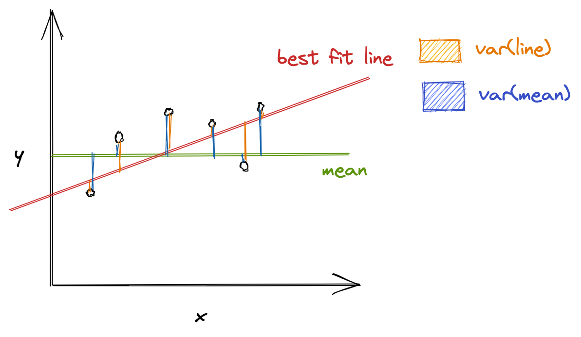
R-squared (also called the coefficient of determination) represents the goodness-of-fit measure for regression models. It gives the proportion of variance in the target variable (dependent variable) that the independent variables explain collectively.

R-squared evaluates the scatter of data points around the best fit line. It can be formulated as:

\[ R^2 = \frac{var(mean) - var(line)}{var(mean)} \]

where \( var(mean) \) is the variance with respect to mean, and var(line) is the variance concerning the best fit line. The \( R^2 \) value can help relate \( var(mean) \) against the \( var(line) \). If \( R^2 \) is, say, 0.83, it means that there is 83% less variation around the line than the mean, i.e., the relationship between independent variables and the target variable accounts for 83% of the variation³.

The higher the R-squared value, the better the model. 0% means that the model does not explain any variance of the target variable around its mean, whereas 100% means that the model explains all variations in the target variable around its mean.

RMSE vs. R Squared

It’s better to compute both the metrics because RMSE calculates the distance between predicted and observed values, whereas, R-squared tells how well the predictor variables (the data attributes) can explain the variation in the target variable.

Limitations

R-squared doesn’t always present an accurate value to conclude if the model is good. For example, if the model is biased, R-squared can be pretty high, which isn’t reflective of the biased data. Hence, it is always advisable to use R-squared with other stats and residual plots for context⁴.

Evaluation Metrics for Classification

Classification is a technique to identify class labels for a given dataset. Consider a scenario where you want to classify an automobile as excellent/good/bad. You then could train a model on a dataset containing information about both the automobile of interest and other classes of vehicle, and verify the model is effective using classification metrics to evaluate the model's performance. To analyze the credibility of your classification model on test/validation datasets, techniques that you can use are as follows:

Accuracy

Accuracy is the percentage of correct predictions for the test data. It is computed as follows:

\[ accuracy = \frac{correct\, predictions}{all\, predictions} \]

In classification, the meta metrics we usually use to compute our metrics are:

• True Positives (TP): Prediction belongs to a class, and observed belongs to a class as well
• True Negatives (TN): Prediction doesn’t belong to a class and observation doesn’t belong to that class
• False Positives (FP): Prediction belongs to a class, but observation doesn’t belong to that class
• False Negatives (FN): Prediction doesn’t belong to a class, but observation belongs to a class

All meta metrics can be arranged in a matrix as follows:

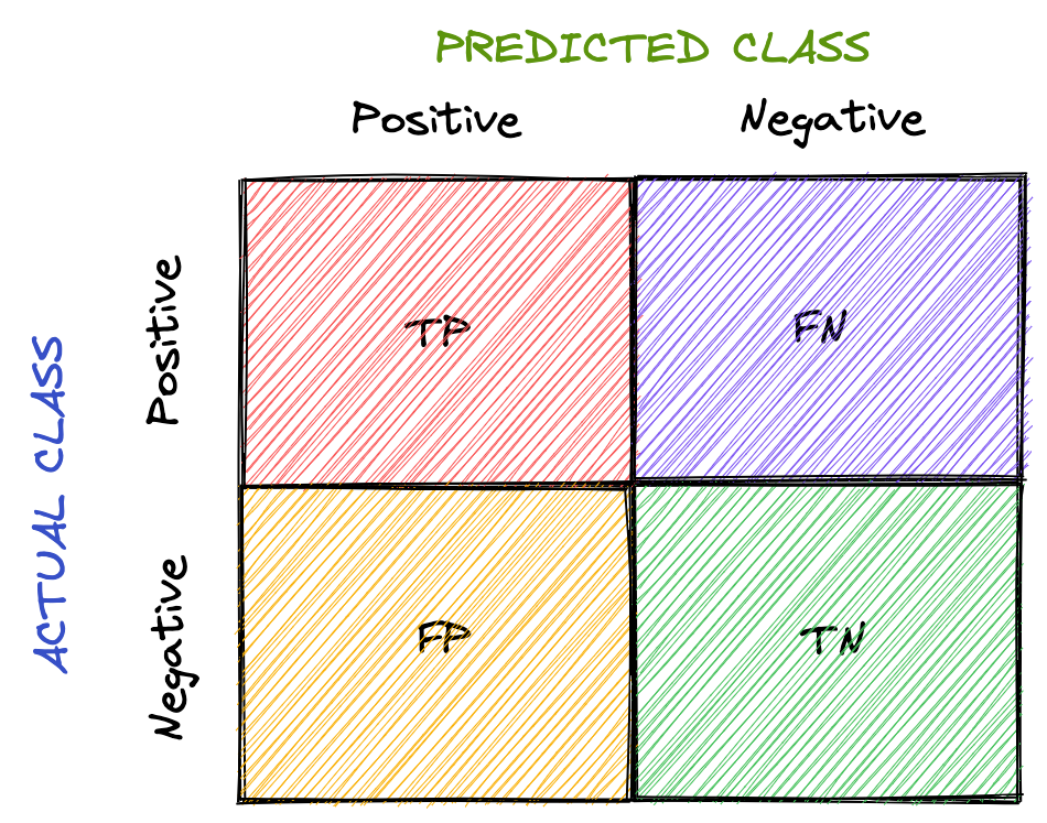
This is called the confusion matrix. It gives a visual representation of the algorithm's performance.

For multiclass classification, we would have more rows and columns, denoting the dataset's classes.

Now let’s rework our accuracy formula using the meta metrics.

\[ accuracy = \frac{TP + TN}{TP + TN + FP + FN} \]

\( TP + TN \) is used because \( TP + TN \) together denote the correct predictions.

Limitations

Accuracy might not always be a good performance indicator. For example, in the case of cancer detection, the cost of failing to diagnose cancer is much higher than the cost of diagnosing cancer in a person who doesn’t have cancer. If the accuracy here is said to be 90%, we are missing out on the other 10% who might have cancer.

Overall, accuracy depends on the problem in consideration. Along with accuracy, you might want to think about other classification metrics to evaluate your model.

Precision

Precision is defined as the fraction of correctly classified samples among all data points that are predicted to belong to a certain class. In general, it translates to “how many of our predictions to belong to a certain class are correct”.

\[ precision = \frac{TP}{TP + FP} \]

To understand precision, let’s consider the cancer detection problem again. If “having cancer” is a positive class, meta metrics are as follows:

\( TP \) = prediction: having cancer, actual (observed): having cancer

\( FP \) = prediction: having cancer, actual: not having cancer

Thus, \( \frac{TP}{TP + FP} \) gives the measure of how well our prediction fares, i.e., it measures how many people diagnosed with cancer have cancer and helps ensure we don’t misclassify people not having cancer as having cancer.

Recall

Recall (also called sensitivity) is defined as the fraction of samples predicted to belong to a class among all data points that actually belong to a class. In general, it translates to “how many data points that belong to a class are correctly classified”.

\[ recall = \frac{TP}{TP + FN} \]

Considering the cancer detection problem, if “having cancer” is a positive class, meta metrics are as follows:

\( TP \): prediction: having cancer, actual (observed): having cancer

\( FN \): prediction: not having cancer, actual: having cancer

Thus, \( \frac{TP}{TP + FN} \) measures how well classification has been done with respect to a class, i.e., it measures how many people with cancer are diagnosed with cancer, and helps ensure that cancer doesn’t go undetected.

F-Measure

Since precision and recall capture different properties of the model, it’s sometimes beneficial to compute both metrics together. In situations where both metrics bear consideration, how about we have precision and recall in a single metric?

F-Measure (also called F1-Measure) comes to the rescue. It is the harmonic mean of precision and recall.

\[ F-Measure = \frac{2}{\frac{1}{recall} + \frac{1}{precision}} = 2 * \frac{precision * recall}{precision + recall} \]

A generalized F-measure is \( F_\beta \), which is given as:

\[ F_\beta = (1 + \beta ^2) * \frac{precision * recall}{(\beta^2 * precision) + recall} \]

where \( \beta \) is chosen such that recall is considered \( \beta \) times as important as precision⁵.

Specificity

Specificity is defined as the fraction of samples predicted to not belong to a class among all data points that actually do not belong to a class. In general, it translates to “how many data points that do not belong to a class are correctly classified”.

\[ specificity = \frac{TN}{TN + FP} \]

Considering the cancer detection problem, if “having cancer” is a positive class, meta metrics are as follows:

\( TN \): prediction: not having cancer, actual (observed): not having cancer

\( FP \): prediction: having cancer, actual: not having cancer

Thus, \( \frac{TN}{TN + FP} \) measures how well classification has been done with respect to a class, i.e., it measures how many people not having cancer are predicted as not having cancer.

ROC

The receiver operating characteristic (ROC) curve plots recall (true positive rate) and false-positive rate.  

\[ TPR = \frac{TP}{TP + FN} \]

\[ FPR = \frac{FP}{FP + TN} \]

The area under ROC (AUC) measures the entire area under the curve. The higher the AUC, the better the classification model.

For example, if the AUC is 0.8, it means there is an 80% chance that the model will be able to distinguish between positive and negative classes.

PR

The precision-recall (PR) curve plots precision and recall. When it comes to imbalanced classification, the PR curve could be helpful. The resulting curve could belong to any of the following tiers:

• High precision and recall: A higher area under the PR curve indicates high precision and recall, which means that the model is performing well by generating accurate predictions (precision: model detects cancer; indeed, has cancer) and correctly classifying samples belonging to a certain class (recall: has cancer, accurately diagnoses cancer).
• High precision and low recall: The model detects cancer, and the person indeed has cancer; however, it misses a lot of actual "has cancer" samples.
• Low precision and high recall: The model gives a lot of "has cancer" and "not having cancer" predictions. It thinks a lot of "has cancer" class samples as "not having cancer"; however, it also misclassifies many "has cancer" when "not having cancer" is the suitable class.
• Low precision and low recall: Neither the classification is done right, nor the samples belonging to a specific class are predicted correctly.

ROC vs. PR

• ROC curve can be used when the dataset is not imbalanced because despite the dataset being imbalanced, ROC presents an overly optimistic picture of the model's performance
• PR curve should be used when the dataset is imbalanced

In this article, you got to know several evaluation metrics that can evaluate regression and classification models.

The caveat here could be that not every evaluation metric can be independently relied on; to conclude if a model is performing well, we may consider a group of metrics.

Besides evaluation metrics, the other measures that one could focus on to check if an ML model is acceptable include:

• Compare your model's score with other similar models and verify if your model's performance is on par with them
• Keep an eye out for Bias and variance to verify if a model generalizes well
• Cross-validation

In the next part, let's dig into the evaluation metrics for clustering and ranking models.

Notebooks detailing the material covered above can be found on Github here.