The first part of this series covered regression and classification evaluation metrics. Here in the part two, let's try and understand the clustering and ranking evaluation metrics.
Evaluation Metrics for Clustering
To find similarities between data points that have no associated class labels, clustering can be used. It divides the data points into multiple clusters such that data points within the same cluster are more similar to each other than the data points within other clusters.
Clustering, being an unsupervised learning technique, doesn’t itself provide a reasonable way to determine the veracity of models. To ameliorate this problem, several approaches have been developed. These techniques include1:
- Internal Evaluation: Internal evaluation is based on the data that is clustered, which includes computing the inter- and intra-cluster distances. The best score is assigned to a model if there is a high similarity within the inter-cluster points and a low similarity between intra-cluster points.
- External Evaluation: External evaluation is based on data not used for clustering, which could include external benchmarks.
- Manual Evaluation: Manual evaluation is done by a human expert.
Let’s now look at a few internal and external evaluation metrics. For worked examples of the different evaluation metrics below, you can follow along in this Gradient Notebook by forking it, or look at it directly on Github.
Bring this project to life
Silhouette Coefficient
The silhouette coefficient (internal evaluation technique) is calculated for each data point using mean intra-cluster distance and mean inter-cluster distance.
\[ silhouette\, coefficient = \frac{b-a}{max(a,b)} \]
\( a \) = mean distance between the current data point and all other data points in the same cluster.
\( b \) = mean distance between the current data point and all other data points in the next nearest cluster.
The silhouette coefficient varies between -1 to 1, with -1 indicating that the data point isn’t assigned to the right cluster, 0 indicating that the clusters are overlapping, and 1 indicating that the cluster is dense and well-separated (this is thus the desirable value).
The closer the value is to 1, the better the clustering method.
Dunn Index
Dunn Index (internal evaluation technique) is useful to identify sets of clusters that are compact and have small variance between the members of the cluster.
\[ Dunn\, Index = \frac{\underset{1 \leq i \lt j \leq c}{min} \delta(x_i, y_j)}{\underset{1 \leq k \leq c}{max} \Delta(x_k)} \]
- \( \delta(x_i, y_j) \) is the inter-cluster distance, i.e., the distance between \( x_i \) and \( x_j \). Internally, it involves computing the distance between every data point in the two clusters. We will have to use the minimum of these distances as the inter-cluster separation.
- \( \Delta_k \) is the intra-cluster distance of cluster \( x_k \), i.e., the distance within the cluster \( x_k \), which involves computing the distance between every data point to every other data point in the same cluster. We will have to consider the maximum of these distances as the intra-cluster separation.
The higher the Dunn index, the better the clustering model.
Davies-Bouldin Index
Davies-Bouldin Index (internal evaluation technique) can be calculated as follows:
\[ Davies-Bouldin\, Index = \frac{1}{c} \sum_{i=1}^{c} \underset{j \neq i}{max} \frac{\sigma_i + \sigma_j}{d(c_i, c_j)} \]
where \( c \) is the number of clusters, \( c_i \) is the centroid of cluster \( i \) , \( d(c_i, c_j) \) is the distance between centroids of two clusters, and \( \sigma_i \) is the average distance of all data points in cluster \( i \) to \( c_i \).
Models that give low intra-cluster distances and high inter-cluster distances (desired metrics!) output a low Davies-Bouldin Index.
Thus, the lower the Davis-Bouldin Index, the better the model.
Calinski-Harabasz Index
Calinski-Harabasz Index (also called variance ratio criterion) (internal evaluation technique) is the ratio between between-cluster dispersion and within-cluster dispersion for all clusters.
\[ CHI = \frac{trace(B_c)}{trace(W_c)} * \frac{n_E - c}{c - 1} \]
where,
\( c \) is the number of clusters,
\( n_E \) is the size of the dataset \( E \),
\( trace(B_c) \) is the trace of between-cluster (inter-cluster) dispersion matrix,
and \( trace(W_c) \) is the trace of within-cluster (intra-cluster) dispersion matrix.
\( W_c \) and \( B_c \) are defined as follows:
\[ W_c = \sum_{i=1}^{c} \sum_{j=1}^{C_i} (x_j - c_i)(x_j - c_i)^T \]
\[ B_c = \sum_{i=1}^{c} n_i (c_i - c_E)(c_i - c_E)^T\]
where \( c \) is the number of clusters, \( C_i \) is the set of data points in cluster \( i\), \( x_j \) is the data point, \( c_i \) is the centroid of cluster \( i \), \( n_i \) is the number of points in cluster \( i \), and \( c_E \) is the global centroid of data \( E \).
Hence, CHI is estimated based on the distances of data points within a cluster from the cluster centroid and distances of all the cluster centroids from the global centroid.
The higher the CHI score, the better the clustering model.
Purity
Purity (external evaluation technique) evaluates the extent to which a cluster belongs to a class. It involves assigning a cluster to a class that is the most frequent in the cluster and then counting the number of correctly assigned data points per cluster, taking the sum over all clusters, and dividing the value by the total number of data points.
\[ Purity = \frac{1}{N} \sum_{c \in C} \underset{d \in D}{max} |c \cap d| \]
where \( C \) refers to clusters, \( D \) refers to classes, and \( N \) is the total number of data points.
A purity of 1 indicates good clustering and purity of 0 indicates bad clustering. The higher the number of clusters, the easier it is to have a high purity value (consider the case when every data point is in its own cluster; it gives a purity of 1!).
Limitations
Purity doesn’t really work well with imbalanced data. Also, purity cannot be used to trade off the clustering quality against the number of clusters since purity is high in the presence of more clusters2.
Normalized Mutual Information
Normalized Mutual Information (NMI) (external evaluation technique) is a normalization of the Mutual Information (MI) score to scale the results between 0 (no mutual information) and 1 (perfect correlation)⁷. It is given as follows:
\[ NMI(\Omega, C) = \frac{I(\Omega;C)}{\frac{H(\Omega) + H(C)}{2}} \]
\( I(\Omega; C) \) represents mutual information. It measures the amount of information by which our knowledge about the class increases when we are told about the clusters3.
\( I(\Omega; C)=0 \) indicates we do not know which class a cluster maps to.
\( I(\Omega; C)=1 \) indicates that every cluster is mapped to a class.
Every data point belonging to its own cluster has a higher \( I(\Omega; C) \) (as in purity). To attain the tradeoff mentioned earlier in Purity, \( \frac{H(\Omega) + H(C)}{2} \) is helpful. \( H \) (entropy) increases as the number of clusters increases, thus keeping \( I(\Omega; C) \) in check.
Rand Index
The Rand Index (RI) (external evaluation technique) measures the percentage of correct predictions among all predictions.
\[ RI = \frac{TP + TN}{TP + TN + FP + FN} \]
The metrics are computed against the benchmark classifications, i.e., \( TP \) is the number of pairs of points clustered together in predicted partition and ground truth partition4, etc.
Rand index ranges from 0 to 1, with 1 indicating a good clustering model.
Limitations
The rand index weighs false positives (FP) and false negatives (FN) equally, which may be an undesirable characteristic for some clustering procedures. To tackle this problem, F-Measure can be used.
Adjusted Rand Index
Adjusted Rand Index (ARI) (external evaluation technique) is the corrected-for-chance version of RI5. It is given using the following formula:
\[ ARI = \frac{RI - Expected\, RI}{Max(RI) - Expected\, RI} \]
ARI establishes a baseline by using expected similarity between the clusters. Unlike RI, it can yield negative values if \( RI \) is less than \( Expected\, RI \).
Jaccard Index
The Jaccard Index (external evaluation technique) measures the number of true positives (TP) against TP, FP, and FN.
\[ JI = \frac{TP}{TP + FP + FN} \]
Given that this simplistic measure looks at the ratio of correct predictions over true positive + all false predictions, a higher ratio indicates a large amount of similarity between the values in the two clusters. The higher the Jaccard index, the better the clustering model.
Limitations
The Jaccard index is able to capably measure similarity between the two groups, but is susceptible to potentially misunderstanding the relationship between the two clusters. For example, one cluster could exist within another, but still be clearly delineated into two distinctly separate clusters.
Bring this project to life
Evaluation Metrics for Ranking
When the order of predictions matters, ranking can be used. Consider a scenario where web pages need to be retrieved in a specific order against a user-given query during Google search. The training data typically consists of a list of web pages or documents against which relevancy is given; the more the relevancy, the higher its rank.
If building such a model, some evaluation metrics that can be used are as follows:
Precision@n
Precision is defined as the fraction of correctly classified samples among all data points that are predicted to belong to a certain class. Precision@n is the precision evaluated until the \( n_{th} \) prediction.
\[ Precision@n = \frac{TP@n}{TP@n + FP@n} \]
Precision@n helps identify the relevant predictions amongst the top \( n \) predictions.
Limitations
Precision@n doesn’t consider the positions of the ordered predictions.
Average Precision
Average Precision (AP) tells us how many relevant predictions are present in the highest-ranked predictions. It can be computed using the following algorithm:
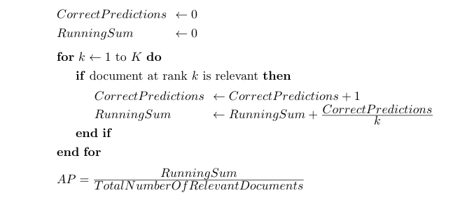
In terms of precision, it is given as:
\[ AP = \frac{\sum_{i=1}^{k} P(k) * rel(k)}{number\, of\, relevant\, documents} \]
where \( P(k) \) is the precision until \( k \) and \( rel(k) \) is the relevance of the \( k^{th}\) prediction.
Mean Average Precision
Mean Average Precision (mAP) is the mean of average precisions against all examples (queries in web search).
\[ mAP = \frac{1}{N} \sum_{i=1}^{N} AP_i\]
\( N \) is the number of queries.
mAP helps evaluate the score not just against a single example, but a set of them.
Discounted Cumulative Gain
Discounted Cumulative Gain (DCG) measures the usefulness of a prediction based on its position in the result list. The premise of DCG is that highly relevant documents appearing lower in a search result list should be penalized as the graded relevance value is reduced logarithmically proportional to the position of the result6.
\[ DCG_k = \sum_{i=1}^{k} \frac{rel_i}{log_2(i+1)} \]
\(k \) is the number until which DCG is accumulated and \( rel_i \) is the relevance of a prediction (web page/document in web search).
Normalized Discounted Cumulative Gain
To normalize DCG values that could vary depending on the number of results per query, Normalized Discounted Cumulative Gain (nDCG) can be used. nDCG uses Ideal DCG (IDCG) to normalize DCG. IDCG is the best possible DCG.
\[ nDCG_k = \frac{DCG_k}{IDCG_k} \]
\(k \) is the number until which nDCG is accumulated.
If the ranking algorithm is perfect, nDCG would be 1 with DCG equal to IDCG.
DCG & NDCG Limitations
DCG & NDCG are the most commonly used ranking evaluation metrics. However, they do not consider the predictions above the current prediction (highly-ranked); hence, the gain at a particular position always remains the same.
Mean Reciprocal Rank
Mean Reciprocal Rank (MRR) computes the mean of the inverse of ranks at which the first relevant prediction is seen for a set of queries, i.e., if, for a given query, the relevant prediction is at the first position, then the relative rank is \( \frac{1}{1} \), for the second position, the relative rank is \( \frac{1}{2} \), and so on. When relative ranks are computed against a set of queries, it results in MRR.
\[ MRR = \frac{1}{|N|} \sum_{i=1}^{|N|} \frac{1}{rank_i} \]
where \( rank_i \) is the position of the relevant prediction and \( N \) is the number of queries.
Limitations
MRR only considers the rank of the first relevant prediction. This isn’t a good choice if more than one relevant prediction should be present high on the predictions.
Kendall’s Tau and Spearman’s Rho
Kendall’s tau (\( \tau \)) and Spearman’s rho (\( \rho \)) are the statistical measures that determine the relationship between ranked data (say, when ranked predictions need to be compared with ranked observations).
Kendall’s Tau is given by the following formula:
\[ \tau = \frac{number\, of\, concordant\, pairs - number\, of\, discordant\, pairs}{\binom{n}{2}} \]
where \( \binom{n}{2} \) is equal to \( \frac{n(n-1)}{2} \)—number of ways to choose two items from \( n \) items.
Concordant pairs: The prediction pairs which are in the same order, i.e., the pairs are ordered equally higher or lower.
Discordant pairs: The prediction pairs that aren’t in the same order, or those ranked in opposite directions.
Spearman’s Rho is given by the following formula:
\[ r_s = \rho_{R(x), R(y)} = \frac{cov(R(X), R(Y))}{\sigma_{R(X)} \sigma_{R(Y)}} \]
where,
\( \rho \) is the Pearson correlation coefficient,
\( cov(R(X),R(Y)) \) is the covariance of rank variables (or ranks),
\( \sigma_{R(X)} \) and \( \sigma_{R(Y)} \) are the standard deviations of the rank variables.
If the ranks are distinct integers, Spearman’s Rho can be computed as:
\[ r_s = 1 - \frac{6 \sum d_i^2}{n(n^2 -1)} \]
where \( d \) is the difference between ranks and \( n \) pertains to the number of ranks.
Conclusion
Through evaluation, we can derive conclusions such as:
- Is the model able to learn from data, rather than memorizing it?
- How would the model perform in real-time scenarios on practical use cases?
- How well is the model doing?
- Does the training strategy have to be improved?
Do we need more data, more features, a different algorithm altogether, etc.?
In this article series, we got to know several evaluation metrics that can evaluate clustering and ranking models.
Evaluating an ML model is an essential parameter to decide if a model's performance is good. As discussed above, a myriad of evaluation metrics for ML and DL models exist. We have to choose the right technique while actively considering the type of model, dataset, and use case. Often, a single metric will not suffice. In such a case, one could use a combination of metrics.
I hope you enjoyed reading the evaluation metrics series!