While many recent advancements in deep neural networks have inclined towards prioritizing performance over complexity, there is still a spark in the community to make deep neural networks cheaper and more efficient for use on smaller devices. There have been various directions of research into efficient neural networks, ranging from Binary Neural Networks and Efficient Networks to component-based research like PyConv and Depthwise Convolution Layers. One work that has stood the test of time is the collection of MobileNet models, which include MobileNet, MobileNetV2, and MobileNetV3.
In this post, we will continue with advancements in the MobileNet range of models with the new entry of MobileNeXt, which was published at ECCV 2020. We will first review the bottleneck structures of Residual Networks and MobileNetV2, and discuss their differences. Next, we will present the redesigned bottleneck structure proposed in MobileNeXt, before diving into the PyTorch implementation of the SandGlass block. We will conclude this article by going through the results as observed in the paper, followed by the model's shortcomings.
Bring this project to life
Table of Contents
- Abstract
- Bottleneck Structures
- Main Branch
- Residual Connection
- Inverted Residual Connections
- MobileNeXt
- SandGlass Block
- PyTorch Code
- Results
- ImageNet Classification
- Object Detection on PASCAL VOC
- Shortcomings and Further Comments
- References
Abstract
- Our results advocate a rethinking of the bottleneck structure for mobile network design. It seems that the inverted residuals are not so advantageous over the bottleneck structure as commonly believed.
- Our study reveals that building shortcut connections along higher-dimensional feature space could promote model performance. Moreover, depthwise convolutions should be conducted in the high dimensional space for learning more expressive features and learning linear residuals is also crucial for bottleneck structure.
- Based on our study, we propose a novel sandglass block, which substantially extends the classic bottleneck structure. We experimentally demonstrate that this structure is more suitable for mobile applications in terms of both accuracy and efficiency and can be used as ‘super’ operators in architecture search algorithms for better architecture generation.
Bottleneck Structures
The first major advent towards high-performing neural network architectures was undoubtedly the Residual Network (referred to as ResNet). Residual Networks have been the staple and bible of modern neural network architectures. The residual layer proposed in these networks has been present in all novel architectures because of its ability to improve information propagation.
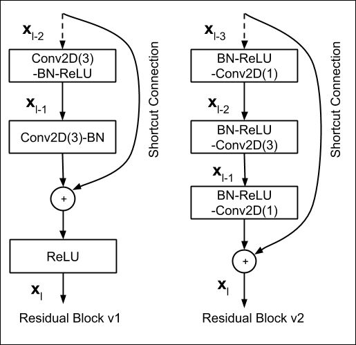
ResNet proposed an underlying fundamentally portable structure called the Residual Block. There are two variants of the Residual Block, as shown in the above diagram; Residual Block v1 and Residual Block v2. Residual Block v1 is predominately used for the smaller ResNet models evaluated on CIFAR datasets, while the Residual Block v2 is the more discussed block structure used for ImageNet-based models. From now on, when we mention the Residual block, we will be referring to the Residual Block v2 to keep the discussion relevant to ImageNet-based models.
Let's dissect this Residual Bottleneck into its core components, which include the main branch and the residual connection (also referred to as the "shortcut connection").
Main Branch
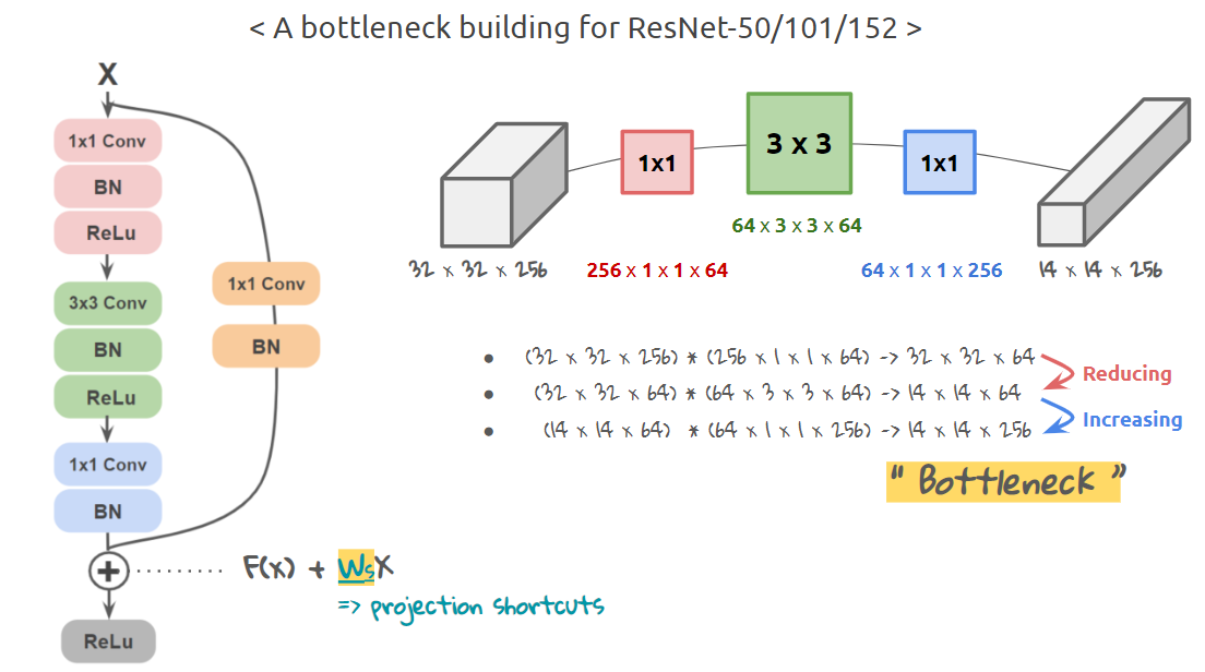
As shown above, in a Residual Block the input first undergoes a $(1 \times 1)$ pointwise convolution operator (note: pointwise convolution doesn't affect the spatial dimensions of the input tensor, but is used to manipulate the number of channels in the tensor). This is followed by a channel-preserving spatial $(3 \times 3)$ convolution which essentially reduces the spatial dimensions of the feature maps in the input tensor. Finally, this is followed by another pointwise $(1 \times 1)$ convolution layer which increases the number of channels to the same number as that of the input to the main branch.
Residual Connection
Parallel to the main branch, the input tensor is projected to the same dimensions as that of the output of the main branch. The only dimension that the input needs to be altered for the residual connections is the spatial dimension, which is achieved by using a $(1 \times 1)$ convolution operator with an increased stride to match the spatial dimension with that of the output of the main branch. (Note: this $(1 \times 1)$ convolution is not a pointwise operator.)
Following this, the residual is added to the main branch output before finally being passed through the standard non-linear activation function (in this case, ReLU).
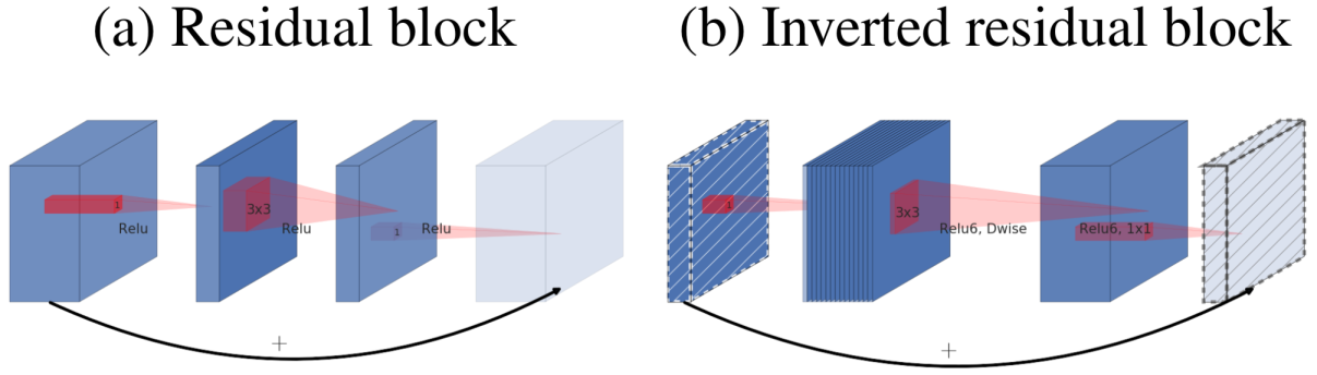
Inverted Residual Connections
MobileNeXt
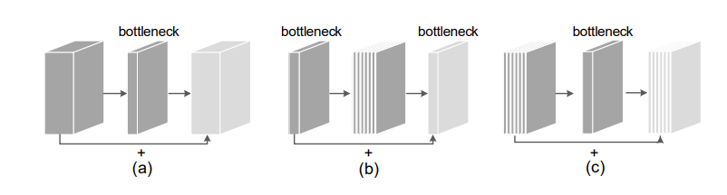
Dethroning its predecessor MobileNetV1, MobileNetV2 proved to be one of the most widely used lightweight architectures by introducing the Inverted Residual Block. While the Residual Block connected the higher dimensional tensors (i.e. those with more channels) via a residual/shortcut connection, MobileNetV2 proposed to invert this by connecting the bottlenecks via the residual connection and keeping the larger channel tensors within the main branch. This was one of the crucial redesign factors in reducing the parameters and FLOPs required.
This was further amplified by the usage of Depthwise Convolution layers, which essentially have one convolutional filter per channel. With this structural overhaul, MobileNets weren't able to outperform their ResNet counterparts in performance metrics like Top-1 accuracy on the ImageNet dataset (which was largely due to the fact that, because of the usage of depthwise convolution operators, the feature space reduced dramatically and thus the expressivity reduced considerably. MobileNet was still able to achieve respectable performance considering how lightweight, fast, and efficient it is compared to the ResNet line of models).
SandGlass Block
Building on our previous discussion of Bottleneck structures, MobileNeXt essentially proposed yet another overhaul of the Bottleneck structure which they call the SandGlass block (shown in the image above). Abstractly, SandGlass is a simple combination of the classic Residual Bottleneck and the Inverted Residual Bottleneck, where it incorporates the best of both worlds. Let's look at it in more detail:
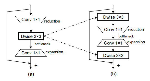
The SandGlass Block is essentially a classic Residual Block, where the first and last convolutional layers in the main branch are channel preserving spatial depthwise convolutional layers. To emulate the bottleneck structure, it uses two consecutive pointwise convolution operators to initially reduce and then subsequently increase the number of channels. These pointwise operators are stacked in between the two depthwise convolution layers. Because of the now larger channel tensors being operated by depthwise kernels, there is a substantial decrease in the number of parameters as compared to e.g. MobileNetV2.
PyTorch Code
import math
import torch
from torch import nn


def _make_divisible(v, divisor, min_value=None):
    """
    This function is taken from the original tf repo.
    It ensures that all layers have a channel number that is divisible by 8
    It can be seen here:
    https://github.com/tensorflow/models/blob/master/research/slim/nets/mobilenet/mobilenet.py
    :param v:
    :param divisor:
    :param min_value:
    :return:
    """
    if min_value is None:
        min_value = divisor
    new_v = max(min_value, int(v + divisor / 2) // divisor * divisor)
    # Make sure that round down does not go down by more than 10%.
    if new_v < 0.9 * v:
        new_v += divisor
    return new_v


class ConvBNReLU(nn.Sequential):
    def __init__(self, in_planes, out_planes, kernel_size=3, stride=1, groups=1, norm_layer=None):
        padding = (kernel_size - 1) // 2
        if norm_layer is None:
            norm_layer = nn.BatchNorm2d
        super(ConvBNReLU, self).__init__(
            nn.Conv2d(in_planes, out_planes, kernel_size, stride, padding, groups=groups, bias=False),
            norm_layer(out_planes),
            nn.ReLU6(inplace=True)
        )


class SandGlass(nn.Module):
    def __init__(self, inp, oup, stride, expand_ratio, identity_tensor_multiplier=1.0, norm_layer=None, keep_3x3=False):
        super(SandGlass, self).__init__()
        self.stride = stride
        assert stride in [1, 2]
        self.use_identity = False if identity_tensor_multiplier==1.0 else True
        self.identity_tensor_channels = int(round(inp*identity_tensor_multiplier))

        if norm_layer is None:
            norm_layer = nn.BatchNorm2d

        hidden_dim = inp // expand_ratio
        if hidden_dim < oup /6.:
            hidden_dim = math.ceil(oup / 6.)
            hidden_dim = _make_divisible(hidden_dim, 16)

        self.use_res_connect = self.stride == 1 and inp == oup

        layers = []
        # dw
        if expand_ratio == 2 or inp==oup or keep_3x3:
            layers.append(ConvBNReLU(inp, inp, kernel_size=3, stride=1, groups=inp, norm_layer=norm_layer))
        if expand_ratio != 1:
            # pw-linear
            layers.extend([
                nn.Conv2d(inp, hidden_dim, kernel_size=1, stride=1, padding=0, groups=1, bias=False),
                norm_layer(hidden_dim),
            ])
        layers.extend([
            # pw
            ConvBNReLU(hidden_dim, oup, kernel_size=1, stride=1, groups=1, norm_layer=norm_layer),
        ])
        if expand_ratio == 2 or inp==oup or keep_3x3 or stride==2:
            layers.extend([
            # dw-linear
            nn.Conv2d(oup, oup, kernel_size=3, stride=stride, groups=oup, padding=1, bias=False),
            norm_layer(oup),
        ])
        self.conv = nn.Sequential(*layers)

    def forward(self, x):
        out = self.conv(x)
        if self.use_res_connect:
            if self.use_identity:
                identity_tensor= x[:,:self.identity_tensor_channels,:,:] + out[:,:self.identity_tensor_channels,:,:]
                out = torch.cat([identity_tensor, out[:,self.identity_tensor_channels:,:,:]], dim=1)
                # out[:,:self.identity_tensor_channels,:,:] += x[:,:self.identity_tensor_channels,:,:]
            else:
                out = x + out
            return out
        else:
            return out
Results
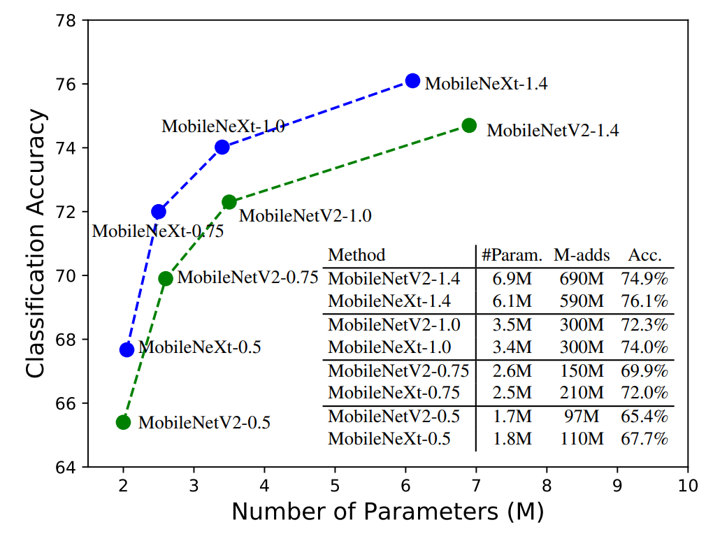
As shown in the graph above, MobileNeXt seems to perform better than MobileNet in every regard. It is lighter in terms of parameters, and still obtains a higher accuracy than its equivalent MobileNetV2 counterpart. In the subsequent tables, we will show how MobileNeXt performs across different tasks, like image classification on the ImageNet dataset and object detection on the Pascal VOC dataset.
ImageNet Classification
| Models | Param. (M) | MAdd (M) | Top-1 Acc. (%) |
|---|---|---|---|
| MobilenetV1-1.0 | 4.2 | 575 | 70.6 |
| ShuffleNetV2-1.5 | 3.5 | 299 | 72.6 |
| MobilenetV2-1.0 | 3.5 | 300 | 72.3 |
| MnasNet-A1 | 3.9 | 312 | 75.2 |
| MobilenetV3-L-0.75 | 4.0 | 155 | 73.3 |
| ProxylessNAS | 4.1 | 320 | 74.6 |
| FBNet-B | 4.5 | 295 | 74.1 |
| IGCV3-D | 7.2 | 610 | 74.6 |
| GhostNet-1.3 | 7.3 | 226 | 75.7 |
| EfficientNet-b0 | 5.3 | 390 | 76.3 |
| MobileNeXt-1.0 | 3.4 | 300 | 74.02 |
| MobileNeXt-1.0† | 3.94 | 330 | 76.05 |
| MobileNeXt-1.1† | 4.28 | 420 | 76.7 |
MobileNeXt† denotes the models with sandglass block and the SE module added for a fair comparison with other state-of-the-art models, such as EfficientNet
Object Detection on PASCAL VOC
| Method | Backbone | Param. (M) | M-Adds (B) | mAP (%) |
|---|---|---|---|---|
| SSD300 | VGG | 36.1 | 35.2 | 77.2 |
| SSDLite320 | MobileNetV2 | 4.3 | 0.8 | 71.7 |
| SSDLite320 | MobileNeXt | 4.3 | 0.8 | 72.6 |
Shortcomings and Further Comments
- The paper failed to provide conclusive results on object detection tasks. It also didn't have MS-COCO experiments to substantially validate its object detection performance.
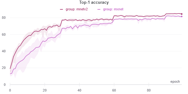
- Since it's more related to the classic Residual Block, it uses the training scheme of ResNets and not that of the MobileNets, and thus is not an apple-to-apple comparison. MobileNeXt performs worse than MobileNetV2 models when tested on CIFAR datasets using the training scheme of MobileNetV2, as shown in the graph below.
Overall, it's a very simple idea yet provides strong results, and it might have a good shot at being the default lightweight model in the computer vision domain.
References
- MobileNetV2: Inverted Residuals and Linear Bottlenecks
- MobileNets: Efficient Convolutional Neural Networks for Mobile Vision Applications
- Searching for MobileNetV3
- ReActNet: Towards Precise Binary Neural Network with Generalized Activation Functions
- EfficientNet: Rethinking Model Scaling for Convolutional Neural Networks
- Pyramidal Convolution: Rethinking Convolutional Neural Networks for Visual Recognition
- Xception: Deep Learning with Depthwise Separable Convolutions
- Rethinking Bottleneck Structure for Efficient Mobile Network Design
- Deep Residual Learning for Image Recognition
- Official Implementation of MobileNeXt
- Unofficial PyTorch implementation of MobileNeXt