‍Implementing Seq2Seq Models for Text Summarization With Keras

So far, we've covered the following in Part 1 of this two-part series:

• Introduction to Seq2Seq Models
• Seq2Seq Architecture and Applications
• Text Summarization Using an Encoder-Decoder Sequence-to-Sequence Model
  • Step 1 - Importing the Dataset
  • Step 2 - Cleaning the Data
  • Step 3 - Determining the Maximum Permissible Sequence Lengths
  • Step 4 - Selecting Plausible Texts and Summaries
  • Step 5 - Tokenizing the Text
  • Step 6 - Removing Empty Text and Summaries

In this tutorial we’ll cover the second part of this series on encoder-decoder sequence-to-sequence RNNs: how to build, train, and test our seq2seq model for text summarization using Keras.

Don't forget that you can follow along with all of the code in this series and run it on a free GPU from a Gradient Community Notebook.

Let's continue!

Step 7: Creating the Model

First, import all the necessary libraries.

from tensorflow.keras.preprocessing.text import Tokenizer
from tensorflow.keras.preprocessing.sequence import pad_sequences
from tensorflow.keras.layers import Input, LSTM, Embedding, Dense, \
    Concatenate, TimeDistributed
from tensorflow.keras.models import Model
from tensorflow.keras.callbacks import EarlyStopping

Next, define the Encoder and Decoder networks.

Encoder

The input length that the encoder accepts is equal to the maximum text length which you’ve already estimated in Step 3. This is then given to an Embedding Layer of dimension (total number of words captured in the text vocabulary) x (number of nodes in an embedding layer)  (calculated in Step 5; the x_voc variable). This is followed by three LSTM networks wherein each layer returns the LSTM output, as well as the hidden and cell states observed at the previous time steps.

Decoder

In the decoder, an embedding layer is defined followed by an LSTM network. The initial state of the LSTM network is the last hidden and cell states taken from the encoder. The output of the LSTM is given to a Dense layer wrapped in a TimeDistributed layer with an attached softmax activation function.

Altogether, the model accepts encoder (text) and decoder (summary) as input and it outputs the summary. The prediction happens through predicting the upcoming word of the summary from the previous word of the summary (see the below figure).

Add the following code to define your network architecture.

latent_dim = 300
embedding_dim = 200

# Encoder
encoder_inputs = Input(shape=(max_text_len, ))

# Embedding layer
enc_emb = Embedding(x_voc, embedding_dim,
                    trainable=True)(encoder_inputs)

# Encoder LSTM 1
encoder_lstm1 = LSTM(latent_dim, return_sequences=True,
                     return_state=True, dropout=0.4,
                     recurrent_dropout=0.4)
(encoder_output1, state_h1, state_c1) = encoder_lstm1(enc_emb)

# Encoder LSTM 2
encoder_lstm2 = LSTM(latent_dim, return_sequences=True,
                     return_state=True, dropout=0.4,
                     recurrent_dropout=0.4)
(encoder_output2, state_h2, state_c2) = encoder_lstm2(encoder_output1)

# Encoder LSTM 3
encoder_lstm3 = LSTM(latent_dim, return_state=True,
                     return_sequences=True, dropout=0.4,
                     recurrent_dropout=0.4)
(encoder_outputs, state_h, state_c) = encoder_lstm3(encoder_output2)

# Set up the decoder, using encoder_states as the initial state
decoder_inputs = Input(shape=(None, ))

# Embedding layer
dec_emb_layer = Embedding(y_voc, embedding_dim, trainable=True)
dec_emb = dec_emb_layer(decoder_inputs)

# Decoder LSTM
decoder_lstm = LSTM(latent_dim, return_sequences=True,
                    return_state=True, dropout=0.4,
                    recurrent_dropout=0.2)
(decoder_outputs, decoder_fwd_state, decoder_back_state) = \
    decoder_lstm(dec_emb, initial_state=[state_h, state_c])

# Dense layer
decoder_dense = TimeDistributed(Dense(y_voc, activation='softmax'))
decoder_outputs = decoder_dense(decoder_outputs)

# Define the model
model = Model([encoder_inputs, decoder_inputs], decoder_outputs)

model.summary()

# Output
Model: "model"
__________________________________________________________________________________________________
Layer (type)                    Output Shape         Param #     Connected to                     
==================================================================================================
input_1 (InputLayer)            [(None, 100)]        0                                            
__________________________________________________________________________________________________
embedding (Embedding)           (None, 100, 200)     5927600     input_1[0][0]                    
__________________________________________________________________________________________________
lstm (LSTM)                     [(None, 100, 300), ( 601200      embedding[0][0]                  
__________________________________________________________________________________________________
input_2 (InputLayer)            [(None, None)]       0                                            
__________________________________________________________________________________________________
lstm_1 (LSTM)                   [(None, 100, 300), ( 721200      lstm[0][0]                       
__________________________________________________________________________________________________
embedding_1 (Embedding)         (None, None, 200)    2576600     input_2[0][0]                    
__________________________________________________________________________________________________
lstm_2 (LSTM)                   [(None, 100, 300), ( 721200      lstm_1[0][0]                     
__________________________________________________________________________________________________
lstm_3 (LSTM)                   [(None, None, 300),  601200      embedding_1[0][0]                
                                                                 lstm_2[0][1]                     
                                                                 lstm_2[0][2]                     
__________________________________________________________________________________________________
time_distributed (TimeDistribut (None, None, 12883)  3877783     lstm_3[0][0]                     
==================================================================================================
Total params: 15,026,783
Trainable params: 15,026,783
Non-trainable params: 0
__________________________________________________________________________________________________

Step 8: Training the Model

In this step, compile the model and define EarlyStopping to stop training the model once the validation loss metric has stopped decreasing.

model.compile(optimizer='rmsprop', loss='sparse_categorical_crossentropy')

es = EarlyStopping(monitor='val_loss', mode='min', verbose=1, patience=2)

Next, use the model.fit() method to fit the training data where you can define the batch size to be 128. Send the text and summary (excluding the last word in summary) as the input, and a reshaped summary tensor comprising every word (starting from the second word) as the output (which explains the infusion of intelligence into the model to predict a word, given the previous word). Besides, to enable validation during the training phase, send the validation data as well.

history = model.fit(
    [x_tr, y_tr[:, :-1]],
    y_tr.reshape(y_tr.shape[0], y_tr.shape[1], 1)[:, 1:],
    epochs=50,
    callbacks=[es],
    batch_size=128,
    validation_data=([x_val, y_val[:, :-1]],
                     y_val.reshape(y_val.shape[0], y_val.shape[1], 1)[:
                     , 1:]),
    )

# Output
Train on 88513 samples, validate on 9835 samples
Epoch 1/50
88513/88513 [==============================] - 426s 5ms/sample - loss: 5.1520 - val_loss: 4.8026
Epoch 2/50
88513/88513 [==============================] - 412s 5ms/sample - loss: 4.7110 - val_loss: 4.5082
Epoch 3/50
88513/88513 [==============================] - 412s 5ms/sample - loss: 4.4448 - val_loss: 4.2815
Epoch 4/50
88513/88513 [==============================] - 411s 5ms/sample - loss: 4.2487 - val_loss: 4.1264
Epoch 5/50
88513/88513 [==============================] - 410s 5ms/sample - loss: 4.1049 - val_loss: 4.0170
Epoch 6/50
88513/88513 [==============================] - 411s 5ms/sample - loss: 3.9968 - val_loss: 3.9353
Epoch 7/50
88513/88513 [==============================] - 412s 5ms/sample - loss: 3.9086 - val_loss: 3.8695
Epoch 8/50
88513/88513 [==============================] - 411s 5ms/sample - loss: 3.8321 - val_loss: 3.8059
Epoch 9/50
88513/88513 [==============================] - 411s 5ms/sample - loss: 3.7598 - val_loss: 3.7517
Epoch 10/50
88513/88513 [==============================] - 410s 5ms/sample - loss: 3.6948 - val_loss: 3.7054
Epoch 11/50
88513/88513 [==============================] - 411s 5ms/sample - loss: 3.6408 - val_loss: 3.6701
Epoch 12/50
88513/88513 [==============================] - 410s 5ms/sample - loss: 3.5909 - val_loss: 3.6376
Epoch 13/50
88513/88513 [==============================] - 411s 5ms/sample - loss: 3.5451 - val_loss: 3.6075
Epoch 14/50
88513/88513 [==============================] - 412s 5ms/sample - loss: 3.5065 - val_loss: 3.5879
Epoch 15/50
88513/88513 [==============================] - 411s 5ms/sample - loss: 3.4690 - val_loss: 3.5552
Epoch 16/50
88513/88513 [==============================] - 409s 5ms/sample - loss: 3.4322 - val_loss: 3.5308
Epoch 17/50
88513/88513 [==============================] - 410s 5ms/sample - loss: 3.3981 - val_loss: 3.5123
Epoch 18/50
88513/88513 [==============================] - 409s 5ms/sample - loss: 3.3683 - val_loss: 3.4956
Epoch 19/50
88513/88513 [==============================] - 409s 5ms/sample - loss: 3.3379 - val_loss: 3.4787
Epoch 20/50
88513/88513 [==============================] - 409s 5ms/sample - loss: 3.3061 - val_loss: 3.4594
Epoch 21/50
88513/88513 [==============================] - 410s 5ms/sample - loss: 3.2803 - val_loss: 3.4412
Epoch 22/50
88513/88513 [==============================] - 409s 5ms/sample - loss: 3.2552 - val_loss: 3.4284
Epoch 23/50
88513/88513 [==============================] - 410s 5ms/sample - loss: 3.2337 - val_loss: 3.4168
Epoch 24/50
88513/88513 [==============================] - 410s 5ms/sample - loss: 3.2123 - val_loss: 3.4148
Epoch 25/50
88513/88513 [==============================] - 409s 5ms/sample - loss: 3.1924 - val_loss: 3.3974
Epoch 26/50
88513/88513 [==============================] - 410s 5ms/sample - loss: 3.1727 - val_loss: 3.3869
Epoch 27/50
88513/88513 [==============================] - 409s 5ms/sample - loss: 3.1546 - val_loss: 3.3853
Epoch 28/50
88513/88513 [==============================] - 408s 5ms/sample - loss: 3.1349 - val_loss: 3.3778
Epoch 29/50
88513/88513 [==============================] - 410s 5ms/sample - loss: 3.1188 - val_loss: 3.3637
Epoch 30/50
88513/88513 [==============================] - 410s 5ms/sample - loss: 3.1000 - val_loss: 3.3544
Epoch 31/50
88513/88513 [==============================] - 413s 5ms/sample - loss: 3.0844 - val_loss: 3.3481
Epoch 32/50
88513/88513 [==============================] - 411s 5ms/sample - loss: 3.0680 - val_loss: 3.3407
Epoch 33/50
88513/88513 [==============================] - 410s 5ms/sample - loss: 3.0531 - val_loss: 3.3374
Epoch 34/50
88513/88513 [==============================] - 410s 5ms/sample - loss: 3.0377 - val_loss: 3.3314
Epoch 35/50
88513/88513 [==============================] - 408s 5ms/sample - loss: 3.0214 - val_loss: 3.3186
Epoch 36/50
88513/88513 [==============================] - 409s 5ms/sample - loss: 3.0041 - val_loss: 3.3128
Epoch 37/50
88513/88513 [==============================] - 410s 5ms/sample - loss: 2.9900 - val_loss: 3.3195
Epoch 38/50
88513/88513 [==============================] - 407s 5ms/sample - loss: 2.9784 - val_loss: 3.3007
Epoch 39/50
88513/88513 [==============================] - 408s 5ms/sample - loss: 2.9655 - val_loss: 3.2975
Epoch 40/50
88513/88513 [==============================] - 410s 5ms/sample - loss: 2.9547 - val_loss: 3.2889
Epoch 41/50
88513/88513 [==============================] - 408s 5ms/sample - loss: 2.9424 - val_loss: 3.2923
Epoch 42/50
88513/88513 [==============================] - 409s 5ms/sample - loss: 2.9331 - val_loss: 3.2753
Epoch 43/50
88513/88513 [==============================] - 411s 5ms/sample - loss: 2.9196 - val_loss: 3.2847
Epoch 44/50
88513/88513 [==============================] - 409s 5ms/sample - loss: 2.9111 - val_loss: 3.2718
Epoch 45/50
50688/88513 [================>.............] - ETA: 2:48 - loss: 2.8809

Next, plot the training and validation loss metrics observed during the training phase.

from matplotlib import pyplot

pyplot.plot(history.history['loss'], label='train')
pyplot.plot(history.history['val_loss'], label='test')
pyplot.legend()
pyplot.show()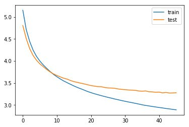

Step 9: Generating Predictions

Now that we've trained the model, to generate summaries from the given pieces of text, first reverse map the indices to the words (which has been previously generated using texts_to_sequences in Step 5). Also, map the words to indices from the summaries tokenizer which is to be used to detect the start and end of the sequences.

reverse_target_word_index = y_tokenizer.index_word
reverse_source_word_index = x_tokenizer.index_word
target_word_index = y_tokenizer.word_index

Now define the encoder and decoder inference models to start making the predictions. Use tensorflow.keras.Model() object to create your inference models.

An encoder inference model accepts text and returns the output generated from the three LSTMs, and hidden and cell states. A decoder inference model accepts the start of the sequence identifier (sostok) and predicts the upcoming word, eventually leading to predicting the whole summary.

Add the following code to define the inference models' architecture.

# Inference Models

# Encode the input sequence to get the feature vector
encoder_model = Model(inputs=encoder_inputs, outputs=[encoder_outputs,
                      state_h, state_c])

# Decoder setup

# Below tensors will hold the states of the previous time step
decoder_state_input_h = Input(shape=(latent_dim, ))
decoder_state_input_c = Input(shape=(latent_dim, ))
decoder_hidden_state_input = Input(shape=(max_text_len, latent_dim))

# Get the embeddings of the decoder sequence
dec_emb2 = dec_emb_layer(decoder_inputs)

# To predict the next word in the sequence, set the initial states to the states from the previous time step
(decoder_outputs2, state_h2, state_c2) = decoder_lstm(dec_emb2,
        initial_state=[decoder_state_input_h, decoder_state_input_c])

# A dense softmax layer to generate prob dist. over the target vocabulary
decoder_outputs2 = decoder_dense(decoder_outputs2)

# Final decoder model
decoder_model = Model([decoder_inputs] + [decoder_hidden_state_input,
                      decoder_state_input_h, decoder_state_input_c],
                      [decoder_outputs2] + [state_h2, state_c2])

Now define a function decode_sequence() which accepts the input text and outputs the predicted summary. Start with sostok and continue generating words until eostok is encountered or the maximum length of the summary is reached. Predict the upcoming word from a given word by choosing the word which has the maximum probability attached and update the internal state of the decoder accordingly.

def decode_sequence(input_seq):

    # Encode the input as state vectors.
    (e_out, e_h, e_c) = encoder_model.predict(input_seq)

    # Generate empty target sequence of length 1
    target_seq = np.zeros((1, 1))

    # Populate the first word of target sequence with the start word.
    target_seq[0, 0] = target_word_index['sostok']

    stop_condition = False
    decoded_sentence = ''

    while not stop_condition:
        (output_tokens, h, c) = decoder_model.predict([target_seq]
                + [e_out, e_h, e_c])

        # Sample a token
        sampled_token_index = np.argmax(output_tokens[0, -1, :])
        sampled_token = reverse_target_word_index[sampled_token_index]

        if sampled_token != 'eostok':
            decoded_sentence += ' ' + sampled_token

        # Exit condition: either hit max length or find the stop word.
        if sampled_token == 'eostok' or len(decoded_sentence.split()) \
            >= max_summary_len - 1:
            stop_condition = True

        # Update the target sequence (of length 1)
        target_seq = np.zeros((1, 1))
        target_seq[0, 0] = sampled_token_index

        # Update internal states
        (e_h, e_c) = (h, c)

    return decoded_sentence

Define two functions - seq2summary() and seq2text() which convert numeric-representation to string-representation of summary and text respectively.

# To convert sequence to summary
def seq2summary(input_seq):
    newString = ''
    for i in input_seq:
        if i != 0 and i != target_word_index['sostok'] and i \
            != target_word_index['eostok']:
            newString = newString + reverse_target_word_index[i] + ' '

    return newString


# To convert sequence to text
def seq2text(input_seq):
    newString = ''
    for i in input_seq:
        if i != 0:
            newString = newString + reverse_source_word_index[i] + ' '

    return newString

Finally, generate the predictions by sending in the text.

for i in range(0, 19):
    print ('Review:', seq2text(x_tr[i]))
    print ('Original summary:', seq2summary(y_tr[i]))
    print ('Predicted summary:', decode_sequence(x_tr[i].reshape(1,
           max_text_len)))
    print '\n'

Here are a few notable summaries generated by the RNN model.

# Output
Review: us president donald trump on wednesday said that north korea has returned the remains of 200 us troops missing from the korean war although there was no official confirmation from military authorities north korean leader kim jong un had agreed to return the remains during his summit with trump about 700 us troops remain unaccounted from the 1950 1953 korean war 
Original summary: start n korea has returned remains of 200 us war dead trump end 
Predicted summary:  start n korea has lost an war against us trump end

Review: pope francis has said that history will judge those who refuse to accept the science of climate change if someone is doubtful that climate change is true they should ask scientists the pope added notably us president donald trump who believes global warming is chinese conspiracy withdrew the country from the paris climate agreement 
Original summary: start history will judge those denying climate change pope end 
Predicted summary:  start pope francis will be in paris climate deal prez end

Review: the enforcement directorate ed has attached assets worth over ã¢â‚â¹33 500 crore in the over three year tenure of its chief karnal singh who retires sunday officials said the agency filed around 390 in connection with its money laundering probes during the period the government on saturday appointed indian revenue service irs officer sanjay kumar mishra as interim ed chief 
Original summary: start enforcement attached assets worth ã¢â‚â¹33 500 cr in yrs end 
Predicted summary:  start ed attaches assets worth 100 crore in india in days end

Review: lok janshakti party president ram vilas paswan daughter asha has said she will contest elections against him from constituency if given ticket from lalu prasad yadav rjd she accused him of neglecting her and promoting his son chirag asha is paswan daughter from his first wife while chirag is his son from his second wife 
Original summary: start will contest against father ram vilas from daughter end 
Predicted summary:  start lalu son tej pratap to contest his daughter in 2019 end


Review: irish deputy prime minister frances fitzgerald announced her resignation on tuesday in bid to avoid the collapse of the government and potential snap election she quit hours before no confidence motion was to be proposed against her by the main opposition party the political crisis began over fitzgerald role in police whistleblower scandal 
Original summary: start irish deputy prime minister resigns to avoid govt collapse end 
Predicted summary:  start pmo resigns from punjab to join nda end

Review: rr wicketkeeper batsman jos buttler slammed his fifth straight fifty in ipl 2018 on sunday to equal former indian cricketer virender sehwag record of most straight 50 scores in the ipl sehwag had achieved the feat while representing dd in the ipl 2012 buttler is also only the second batsman after shane watson to hit two successive 90 scores in ipl 
Original summary: start buttler equals sehwag record of most straight 50s in ipl end 
Predicted summary:  start sehwag slams sixes in an ipl over 100 times in ipl end

Review: maruti suzuki india on wednesday said it is recalling 640 units of its super carry mini trucks sold in the domestic market over possible defect in fuel pump supply the recall covers super carry units manufactured between january 20 and july 14 2018 the faulty parts in the affected vehicles will be replaced free of cost the automaker said n 
Original summary: start maruti recalls its mini trucks over fuel pump issue in india end 
Predicted summary:  start maruti suzuki recalls india over ã¢â‚â¹3 crore end

Review: the arrested lashkar e taiba let terrorist aamir ben has confessed to the national investigation agency that pakistani army provided him cover firing to infiltrate into india he further revealed that hafiz organisation ud dawah arranged for his training and that he was sent across india to carry out subversive activities in and outside kashmir 
Original summary: start pak helped me enter india arrested let terrorist to nia end 
Predicted summary:  start pak man who killed indian soldiers to enter kashmir end

Review: the 23 richest indians in the 500 member bloomberg billionaires index saw wealth erosion of 21 billion this year lakshmi mittal who controls the world largest steelmaker arcelormittal lost 5 6 billion or 29 of his net worth followed by sun pharma founder dilip shanghvi whose wealth declined 4 6 billion asia richest person mukesh ambani added 4 billion to his fortune 
Original summary: start lakshmi mittal lost 10 bn in 2018 ambani added 4 bn end 
Predicted summary:  start india richest man lost billion in wealth in 2017 end

Conclusion

The Encoder-Decoder Sequence-to-Sequence Model (LSTM) we built generated acceptable summaries from what it learned in the training texts. Although after 50 epochs the predicted summaries are not exactly on par with the expected summaries (our model hasn't yet reached human-level intelligence!), the intelligence our model has gained definitely counts for something.

To attain more accurate results from this model, you can increase the size of the dataset, play around with the hyperparameters of the network, try making it larger, and increase the number of epochs.

In this tutorial, you’ve trained an encoder-decoder sequence-to-sequence model to perform text summarization. In my next article you can learn all about attention mechanisms. Until then, happy learning!

Reference: Sandeep Bhogaraju