In supervised machine learning the training data is already labeled, which means each data instance has its corresponding output(s). In unsupervised machine learning, the data comes without labels. Clustering is an unsupervised learning problem where the task is to explore the data to find the best label for each data instance.
This tutorial discusses how the genetic algorithm is used to cluster data, starting from random clusters and running until the optimal clusters are found. We'll start by briefly revising the K-means clustering algorithm to point out its weak points, which are later solved by the genetic algorithm. The code examples in this tutorial are implemented in Python using the PyGAD library.
The outline of this tutorial is as follows:
- Introduction
- K-Means Clustering
- Clustering Using the Genetic Algorithm
- Preparing Artificial Clustering Data
- Distance to Cluster Centers
- Fitness Function
- Evolution Using the Genetic Algorithm
- Complete Python Code for 2 Clusters
- Example With 3 Clusters
- Conclusion
Bring this project to life
Introduction
Based on whether the training data has labels or not, there are two types of machine learning:
- Supervised learning
- Unsupervised learning
In supervised learning problems, the model uses some information describing the data. This information is the output of the data instances, so that the model knows (and learns) what the expected output should be for each input instance it receives. This helps the model to assess its performance and learn a way to reduce the error (or increase the accuracy).
For a classification problem, the output is the expected class of each sample. For an RGB color classifier, the input and output data can be like the following:
Input  1 : 255, 0, 0
Output 1 : Red

Input  2 : 0, 255, 0
Output 2 : Green
Assume there are just two classes: Red, and Green. When the model knows the expected outputs, it adjusts itself (i.e. its parameters) during the training phase to return the correct outputs. For a new test sample, the model measures its similarity with the samples it saw previously in the two classes.
In unsupervised learning problems, the model does not know the correct outputs for the data (the inputs). Clustering is an unsupervised learning problem where the task is to find the outcome (i.e. label) of each data instance.
The input to the clustering algorithm is just the input as follows:
Input 1 : 255, 0, 0
Input 2 : 0, 255, 0
After clustering, the model should predict the label of each data instance:
Output 1: Red
Output 2: Green
Some clustering algorithms exist, like the K-means algorithm (which is the most popular); branch and bound; and maximum likelihood estimation.
To serve the purpose of this tutorial, which is clustering using the genetic algorithm, the next section reviews the K-means algorithm.
K-Means Clustering
The K-means algorithm is a popular clustering algorithm. Although it is very simple, this section quickly reviews how it works because understanding it is essential to doing clustering using the genetic algorithm.
The inputs to the K-means algorithm are:
- The data samples.
- The number of clusters $K$.
The output of the algorithm is a set of $K$ clusters where each cluster is composed of a set of data samples. One sample may or may not overlap between 2 or more clusters; this depends on the nature of the problem being solved.
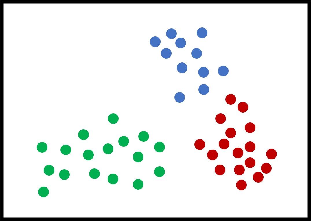
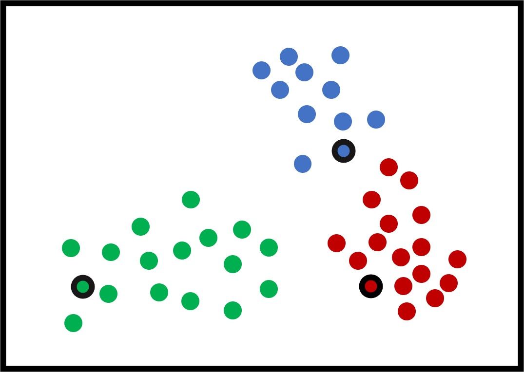
The next figure shows an example with 3 artificial clusters to show how the K-means algorithm works. Note that "artificial" means the data is not real. For this example, it is very clear that the optimal value of $K$ (the best number of clusters) is 3. For real-world problems, different values of $K$ yield different results, and the most feasible one is selected. Each sample has a color that reflects its cluster.
Each cluster could be represented by a set that includes its samples. For example, $C_1={\{32, 21, 5, 2, 9\}}$ means the samples with IDs $32, 21, 5, 2,$ and $9$ belong to the first cluster.
K-means works by selecting an initial center for each of the K clusters. Note that the K-means algorithm is very sensitive to those initial centers and may give different results by changing the initial centers. In the next figure, the selected centers are those with a black border.
The next step is to calculate the distance between each sample and the 3 centers and assign each sample to the cluster of the nearest center. The goal is to minimize the total distance between all samples and their centers. The distance could be the Euclidean distance that is calculated according to the next equation:
$$euc(q, p)=\sqrt{\sum_{i=1}^{F}(C_i-P_i)^2}$$
Where:
- $F$ is the number of features representing each sample.
- $C$ and $P$ are the 2 samples with the Euclidean distance calculated between them.
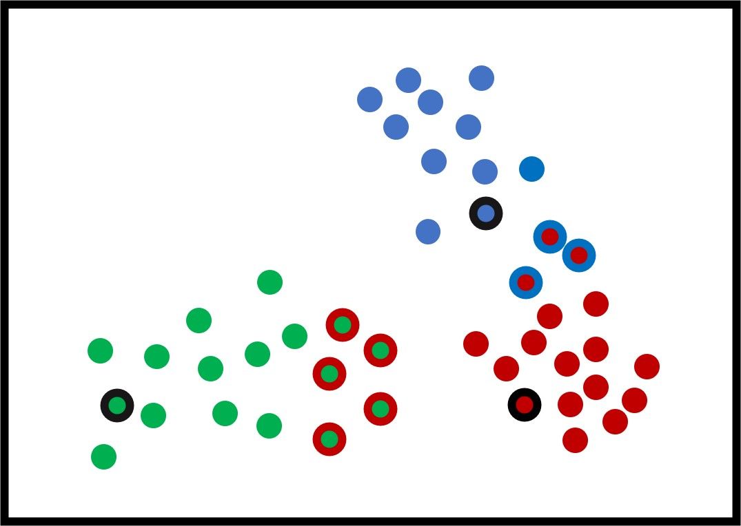
The next figure shows how the samples are clustered. The samples assigned to incorrect clusters have an edge of the same color as the cluster they are mistakenly put inside.
Based on the current clusters, the K-means algorithm updates its $K$ clusters' centers by taking the average of all samples within each cluster according to the next equation:
$$C_icenter=\frac{1}{n_i^k}\sum_{i=1}^{n_i^k}{x_i^k}$$
Where:
- $n$ is the number of samples within the cluster.
- $x_i$ is a sample within the cluster.
If a sample has an equal distance to more than one cluster, then it can be assigned to any of these clusters.
After the new centers are calculated, the cluster centers move from their current locations to other locations that hopefully create new, better clusters. Note that the new cluster center does not need to be a sample from the cluster and may be a new artificial sample.
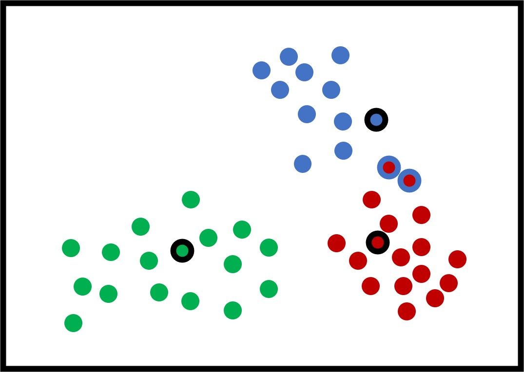
The new figure shows some potential new centers for the clusters. Using these new centers, there are just 2 samples that are within the wrong cluster. Again, the new centers are calculated by averaging all the samples within the cluster.
After updating the centers again, the next figure shows that all the samples are clustered correctly.
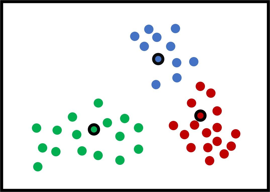
The K-means algorithm continues to generate the new clusters' centers and assign the samples to the cluster with the least distance until it finds that the new centers are exactly identical to the current centers. In this case, the K-means algorithm stops. You can also set it so that the algorithm stops after a certain number of iterations, even if the centers are still changing.
After reviewing how the K-means algorithm works, let's discuss some of its limitations to highlight the benefits of using an evolutionary algorithm, like the genetic algorithm, for clustering.
According to this paper, there are two drawbacks to using K-means clustering:
- The first limitation of the K-means algorithm is that it is very sensitive to the initial centers. Changing the initial centers strongly influences the results.
- The K-means algorithm might fall in the local optima and may not be able to find the globally optimal solution.
One reason why K-means can fall into a local optima is that it stops at the first stable centers, and then has no way to improve them to reach a better solution. K-means has no way to measure the quality of the solution, and it only stops at the first available solution.
These limitations of the K-means algorithm are solved by using the genetic algorithm. The next section shows how the genetic algorithm is used for clustering.
Clustering Using the Genetic Algorithm
The genetic algorithm is an optimization algorithm that searches for a solution for a given problem using a population of more than 1 solution. The genetic algorithm not only searches for a solution, but also searches for the globally optimal solution by making some random (i.e. blind) changes to the solution in multiple directions.
The genetic algorithm follows these steps to find the best solution:
- Initialize a population of solutions.
- Calculate the fitness value of the solutions in the population.
- Select the best solutions (with the highest fitness values) as parents.
- Mate the selected parents using crossover and mutation.
- Create a new population.
- Repeat steps 2 to 5 for a number of generations, or until a condition is met.
For more information about the genetic algorithm, please check out these resources:
- Introduction to Optimization with Genetic Algorithm
- Dan Simon, Evolutionary Optimization Algorithms, Wiley, 2013
For the clustering problem, the genetic algorithm is better than K-means as it is less sensitive to the initial centers. The genetic algorithm does not stop at the first solution, but also evolves it to find the globally optimal solution.
To solve a problem using the genetic algorithm, you have to think of these three things:
- Formulating the problem in the form expected by the genetic algorithm, where each solution is represented as a chromosome.
- Problem encoding (binary or decimal).
- Building a fitness function that measures the fitness (i.e. quality) of the solution.
For clustering problems, the solution to the problem is the center coordinates of the clusters. All of the centers must be represented as a chromosome, which is basically a 1-D vector.
Assume that each sample in the previous problem has just 2 features representing their $X$ and $Y$ location. Assume also that the locations of the 3 clusters are as follows:
$$(C_{1X}, C_{1Y})=(0.4, 0.8)
\space
(C_{2X}, C_{2Y})=(1.3, 2.23)
\space
(C_{3X}, C_{3Y})=(5.657, 3.41)$$
Then the solution should be represented as a 1-D vector as given below, where the first 2 elements are the $X$ and $Y$ locations of the center of the first cluster, the second 2 elements represent the second cluster's center, and so on.
$$(C_{1X}, C_{1Y}, C_{2X}, C_{2Y}, C_{3X}, C_{3Y}) = (0.4, 0.8, 1.3, 2.23, 5.657, 3.41)$$
Because the genes of the solution are already encoded in decimal, using the decimal encoding for the solution is straightforward. If you selected binary encoding, then you must do the following:
- Convert the decimal genes to binary.
- Convert the binary genes to decimal.
In this tutorial, decimal encoding is used to make things simpler.
The Fitness Function
The fitness function is a way of assessing the solution. Because the genetic algorithm uses a maximization fitness function, the goal is to find a solution with the highest possible fitness value.
Inspired by the K-means algorithm, the genetic algorithm calculates the sum of distances between each sample and its cluster center according to the following equation, where the Euclidean distance is used:
$$fitness=\frac{1}{\sum_{k=1}^{N_c}\sum_{j=1}^{N_k}\sqrt{\sum_{i=1}^{F}(C_{ki}-P_{jj})^2}}$$
Where:
- $N_c$ is the number of clusters.
- $N_k$ is the number of samples within the cluster $k$.
- $F$ is the number of features representing the sample, which is 2 in our example.
- $C_k$ is the center of the cluster $k$.
Note how the fitness function uses the inverse of the sum of distances to calculate the fitness. The reason is that using the sum of distances directly makes the fitness function a minimization function, which contradicts the genetic algorithm.
After discussing how clustering using the genetic algorithm works, the remaining parts of this tutorial use Python to do the following:
- Prepare artificial data.
- Cluster the data using the Python library PyGAD.
Prepare the Artificial Clustering Data
This section prepares artificial data to be used in testing the genetic algorithm clustering. The data is selected to have a margin between the different clusters to make things easier at the beginning, and make sure everything is working properly.
Throughout the tutorial, there are 2 sets of artificial data generated. The first set has 2 clusters and the other one has 3 clusters. The data samples are generated randomly, where each sample has only 2 features. Let's focus on the data with just 2 clusters for now.
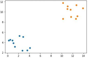
The next code block uses the numpy.random module to randomly generate the data and plot it. Each of the 2 features is scaled in a certain range to make sure the 2 clusters are separated properly. Here are the start and end values used for each of the 2 features in the 2 clusters:
- Cluster 1 Feature 1: (0, 5)
- Cluster 1 Feature 2: (2, 6)
- Cluster 2 Feature 1: (10, 15)
- Cluster 2 Feature 2: (8, 12)
The number of samples within each cluster is set to 10. According to your preference, you can adjust the start and end values of each feature and also the number of samples in each cluster.
import numpy
import matplotlib.pyplot

cluster1_num_samples = 10
cluster1_x1_start = 0
cluster1_x1_end = 5
cluster1_x2_start = 2
cluster1_x2_end = 6
cluster1_x1 = numpy.random.random(size=(cluster1_num_samples))
cluster1_x1 = cluster1_x1 * (cluster1_x1_end - cluster1_x1_start) + cluster1_x1_start
cluster1_x2 = numpy.random.random(size=(cluster1_num_samples))
cluster1_x2 = cluster1_x2 * (cluster1_x2_end - cluster1_x2_start) + cluster1_x2_start

cluster2_num_samples = 10
cluster2_x1_start = 10
cluster2_x1_end = 15
cluster2_x2_start = 8
cluster2_x2_end = 12
cluster2_x1 = numpy.random.random(size=(cluster2_num_samples))
cluster2_x1 = cluster2_x1 * (cluster2_x1_end - cluster2_x1_start) + cluster2_x1_start
cluster2_x2 = numpy.random.random(size=(cluster2_num_samples))
cluster2_x2 = cluster2_x2 * (cluster2_x2_end - cluster2_x2_start) + cluster2_x2_start

matplotlib.pyplot.scatter(cluster1_x1, cluster1_x2)
matplotlib.pyplot.scatter(cluster2_x1, cluster2_x2)
matplotlib.pyplot.show()
Because the data are randomly generated, different results are returned each time the code runs. If you would like to keep the data, save it as .npy files as follows:
numpy.save("p1_cluster1_x1.npy", cluster1_x1)
numpy.save("p1_cluster1_x2.npy", cluster1_x2)
numpy.save("p1_cluster2_x1.npy", cluster2_x1)
numpy.save("p1_cluster2_x2.npy", cluster2_x2)
The next figure shows the samples in each of the 2 clusters, where the samples in the same cluster have the same color.
Note that the single feature in each cluster is in a different array. It is required to group the data samples in all clusters within a single array according to the following code. The arrays c1 and c2 hold the samples of the first and second clusters, respectively. The array data concatenates the c1 and c2 arrays together to hold all the samples of the 2 clusters together. Because each cluster has 10 samples where each sample has 2 features, the shape of the data array is (20, 2).
c1 = numpy.array([cluster1_x1, cluster1_x2]).T
c2 = numpy.array([cluster2_x1, cluster2_x2]).T

data = numpy.concatenate((c1, c2), axis=0)
Because we are looking to cluster the data into 2 clusters, a variable named num_clusters is created to hold the number of clusters.
num_clusters = 2The next section shows how to calculate the Euclidean distance between pairs of samples.
Calculate the Euclidean Distance
The next function named euclidean_distance() accepts 2 inputs X and Y. One of these inputs can be a 2-D array with multiple samples, and the other input should be a 1-D array with just 1 sample. The function calculates and returns the Euclidean distances between each sample in the 2-D array and the single sample in the 1-D array.
def euclidean_distance(X, Y):
    return numpy.sqrt(numpy.sum(numpy.power(X - Y, 2), axis=1))
As an example, the following code calculates the distance between the data samples in the data array and the first sample in that array. Note that it does not matter whether the 2-D array is passed in the first or second argument.
d = euclidean_distance(data, data[0])
# d = euclidean_distance(data[0], data)
print(d)
The result of the euclidean_distance() function is a 1-D array with a number of elements equal to the number of elements in the 2-D array, which is 20 in this example. Because the first element in this array calculates the distance between the first sample and itself, the result is 0.
[ 0.          0.42619051  2.443811    1.87889259  3.75043     1.5822869
  3.96625121  3.06553115  0.86155518  0.28939665 13.96001895 12.06666769
 12.76627205 10.57271874 12.13148125 12.13964431 14.75208149 12.60948923
 12.44900076 13.18736698]
The next section uses the data array and the euclidean_distance() function to calculate the Euclidean distance between each cluster center and all samples to cluster the data. Later, the genetic algorithm will use the calculated distance to evolve the cluster centers.
Distance to Cluster Centers
To use the genetic algorithm for clustering, remember that the fitness function is calculated according to the next equation.
$$fitness=\frac{1}{\sum_{k=1}^{N_c}\sum_{j=1}^{N_k}\sqrt{\sum_{i=1}^{F}(C_{ki}-P_{jj})^2}}$$
To calculate the fitness, the following steps are followed:
- Loop through the cluster centers to calculate the Euclidean distance between all samples and all cluster centers.
- Assign each sample to the cluster with the least Euclidean distance.
- Another loop goes through the clusters to calculate the sum of all the distances in each cluster. If a cluster has 0 samples, then its total distance is 0.
- Sum the distances in all clusters.
- Calculate the inverse of the sum of distances. This is the fitness value.
All of these steps are applied in the cluster_data() function given below. It accepts the following 2 arguments:
solution: A solution from the population to calculate the distance between its centers and the data samples.solution_idx: The index of the solution inside the population.
At the beginning of the function, the following lists are defined:
cluster_centers = []: A list of size(C, f)whereCis the number of clusters andfis the number of features representing each sample.all_clusters_dists = []: A list of size(C, N)whereCis the number of clusters andNis the number of data samples. It holds the distances between each cluster center and all the data samples.clusters = []: A list withCelements where each element holds the indices of the samples within a cluster.clusters_sum_dist = []: A list withCelements where each element represents the sum of distances of the samples with a cluster.
According to our example, the sizes of these arrays are:
cluster_centers = []:(2, 2)all_clusters_dists = []:(2, 20)clusters = []:(2)clusters_sum_dist = []:(2)
The first loop starts from $0$ to the number of clusters, and saves the index of the cluster in the clust_idx variable. For each cluster, the current cluster center is returned from the solution argument and appended to the cluster_centers list.
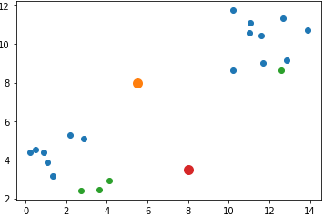
Assume that the initial cluster centers in the solution argument are as follows:
[5.5, 8, 8, 3.5]As a result, the cluster_centers is given below where the center of the first cluster is [5.5, 8] and the center of the second cluster is [8, 3.5].
[[5.5, 8],
 [8 , 3.5]]
The next figure shows the locations of the data samples (in blue and green) and the cluster centers (in orange and red).
import numpy

def cluster_data(solution, solution_idx):
    global num_cluster, data
    feature_vector_length = data.shape[1]
    cluster_centers = []
    all_clusters_dists = []
    clusters = []
    clusters_sum_dist = []

    for clust_idx in range(num_clusters):
        cluster_centers.append(solution[feature_vector_length*clust_idx:feature_vector_length*(clust_idx+1)])
        cluster_center_dists = euclidean_distance(data, cluster_centers[clust_idx])
        all_clusters_dists.append(numpy.array(cluster_center_dists))

    cluster_centers = numpy.array(cluster_centers)
    all_clusters_dists = numpy.array(all_clusters_dists)

    cluster_indices = numpy.argmin(all_clusters_dists, axis=0)
    for clust_idx in range(num_clusters):
        clusters.append(numpy.where(cluster_indices == clust_idx)[0])
        if len(clusters[clust_idx]) == 0:
            clusters_sum_dist.append(0)
        else:
            clusters_sum_dist.append(numpy.sum(all_clusters_dists[clust_idx, clusters[clust_idx]]))

    clusters_sum_dist = numpy.array(clusters_sum_dist)

    return cluster_centers, all_clusters_dists, clusters, clusters_sum_dist
The Euclidean distance between the cluster center and all the data samples is calculated using the euclidean_distance() function, which returns a 1-D array with the distances. The returned 1-D array is appended to the all_clusters_dists list.
According to the centers used, the all_clusters_dists list is given below. For the first data sample, its distance to the first cluster center is 6.10987275 while it is 7.58117358 for the second cluster center. This means the first sample is closer to the first cluster than the second cluster. As a result, it should be assigned to the first cluster.
In contrast, the fifth sample has a distance of 5.87318124 to the first cluster, which is greater than the distance to the second cluster 4.51325553. As a result, the last sample is assigned to the second cluster.
[
    [6.10987275, 5.85488677, 3.92811163, 4.26972678, 5.87318124,
     6.39720168, 5.28119451, 6.24298182, 6.07007001, 6.39430533,
     7.90203904, 6.25946844, 7.09108705, 4.75587942, 6.02754277,
     6.07567479, 8.79599995, 6.58285106, 6.35517978, 7.42091138],

    [7.58117358, 7.1607106 , 5.38161037, 6.08709119, 4.51325553,
     6.69279857, 3.9319092 , 5.39058713, 6.9519177 , 7.82907281,
     9.11361263, 6.63760617, 6.88139784, 5.61260512, 8.54100171,
     7.67377794, 9.30938389, 7.82144838, 8.17728968, 7.42907412]
]
The cluster_centers and all_clusters_dists lists are then converted into NumPy arrays to better handle them.
Based on the distances in the all_clusters_dists list, each sample is assigned to the closest cluster. As given below, the cluster_indices array has a value at each element that corresponds to the assigned cluster of each sample. For example, the first four samples are assigned to the first cluster while the fifth sample is assigned to the second cluster.
array([0, 0, 0, 0, 1, 0, 1, 1, 0, 0, 0, 0, 1, 0, 0, 0, 0, 0, 0, 0])There is another loop that sums the distances of the samples in each cluster. For each cluster, the indices of the samples within it are returned and appended into the clusters list. The next output shows what samples belong to each cluster.
[
 array([ 0,  1,  2,  3,  5,  8,  9, 10, 11, 13, 14, 15, 16, 17, 18, 19]),
 array([ 4,  6,  7, 12])
]
If a cluster has no samples, then its total distance is set to $0$. Otherwise, it is calculated and added to the clusters_sum_dist list. The next output shows the total distance for each cluster.
[99.19972158, 20.71714969]At the end of the cluster_data() function, the following arrays are returned:
cluster_centers: Centers of the clusters.all_clusters_dists: Distances between all samples and all cluster centers.cluster_indices: Index of the cluster the samples are assigned to.clusters: The indices of the samples within each cluster.clusters_sum_dist: Total distance for samples in each cluster.
Fitness Function
A fitness function named fitness_func() is created and calls the cluster_data() function and calculates the sum of distances in all clusters.
The inverse of the sum is calculated to make the fitness function a maximization one.
The tiny value 0.00000001 is added to the denominator in case that the optimal solution is found and the total distance is 0.
def fitness_func(solution, solution_idx):
    _, _, _, _, clusters_sum_dist = cluster_data(solution, solution_idx)

    fitness = 1.0 / (numpy.sum(clusters_sum_dist) + 0.00000001)

    return fitness
This section discussed how the process proceeds from an initial solution of initial cluster centers until calculating their fitness value. The next section uses the genetic algorithm to evolve the cluster centers until reaching an optimal solution.
Evolution Using the Genetic Algorithm
The genetic algorithm can be easily built using the PyGAD library. All you need to do is to create an instance of the pygad.GA class while passing the appropriate parameters. Then, call the run() method to start evolving the cluster centers for a number of generations.
import pygad

num_genes = num_clusters * data.shape[1]
ga_instance = pygad.GA(num_generations=100,
                       sol_per_pop=10,
                       num_parents_mating=5,
                       keep_parents=2,
                       num_genes=num_genes,
                       fitness_func=fitness_func,
                       suppress_warnings=True)

ga_instance.run()

best_solution, best_solution_fitness, best_solution_idx = ga_instance.best_solution()
print("Best solution is {bs}".format(bs=best_solution))
print("Fitness of the best solution is {bsf}".format(bsf=best_solution_fitness))
print("Best solution found after {gen} generations".format(gen=ga_instance.best_solution_generation))
After the run() method completes, some information about the best solution is printed. The next block shows the best solution itself, its fitness, and the generation at which it was found.
Best solution: array([11.630579, 10.40645359, 1.418031, 3.96230158])
Fitness of the best solution is 0.033685406034550607
Best solution found after 73 generations
The next code block uses the best solution found by the genetic algorithm to cluster the data. The figure below shows that the solution adequately clusters the data.
import matplotlib.pyplot

cluster_centers, all_clusters_dists, cluster_indices, clusters, clusters_sum_dist = cluster_data(best_solution, best_solution_idx)

for cluster_idx in range(num_clusters):
    cluster_x = data[clusters[cluster_idx], 0]
    cluster_y = data[clusters[cluster_idx], 1]
    matplotlib.pyplot.scatter(cluster_x, cluster_y)
    matplotlib.pyplot.scatter(cluster_centers[cluster_idx, 0], cluster_centers[cluster_idx, 1], linewidths=5)
matplotlib.pyplot.title("Clustering using PyGAD")
matplotlib.pyplot.show()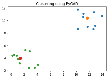
The next GIF shows how the cluster centers evolved from the initial ones to the optimal ones.
Complete Code for Two Clusters
import numpy
import matplotlib.pyplot
import pygad

cluster1_num_samples = 10
cluster1_x1_start = 0
cluster1_x1_end = 5
cluster1_x2_start = 2
cluster1_x2_end = 6
cluster1_x1 = numpy.random.random(size=(cluster1_num_samples))
cluster1_x1 = cluster1_x1 * (cluster1_x1_end - cluster1_x1_start) + cluster1_x1_start
cluster1_x2 = numpy.random.random(size=(cluster1_num_samples))
cluster1_x2 = cluster1_x2 * (cluster1_x2_end - cluster1_x2_start) + cluster1_x2_start

cluster2_num_samples = 10
cluster2_x1_start = 10
cluster2_x1_end = 15
cluster2_x2_start = 8
cluster2_x2_end = 12
cluster2_x1 = numpy.random.random(size=(cluster2_num_samples))
cluster2_x1 = cluster2_x1 * (cluster2_x1_end - cluster2_x1_start) + cluster2_x1_start
cluster2_x2 = numpy.random.random(size=(cluster2_num_samples))
cluster2_x2 = cluster2_x2 * (cluster2_x2_end - cluster2_x2_start) + cluster2_x2_start

c1 = numpy.array([cluster1_x1, cluster1_x2]).T
c2 = numpy.array([cluster2_x1, cluster2_x2]).T

data = numpy.concatenate((c1, c2), axis=0)

matplotlib.pyplot.scatter(cluster1_x1, cluster1_x2)
matplotlib.pyplot.scatter(cluster2_x1, cluster2_x2)
matplotlib.pyplot.title("Optimal Clustering")
matplotlib.pyplot.show()

def euclidean_distance(X, Y):
    return numpy.sqrt(numpy.sum(numpy.power(X - Y, 2), axis=1))

def cluster_data(solution, solution_idx):
    global num_cluster, data
    feature_vector_length = data.shape[1]
    cluster_centers = []
    all_clusters_dists = []
    clusters = []
    clusters_sum_dist = []

    for clust_idx in range(num_clusters):
        cluster_centers.append(solution[feature_vector_length*clust_idx:feature_vector_length*(clust_idx+1)])
        cluster_center_dists = euclidean_distance(data, cluster_centers[clust_idx])
        all_clusters_dists.append(numpy.array(cluster_center_dists))

    cluster_centers = numpy.array(cluster_centers)
    all_clusters_dists = numpy.array(all_clusters_dists)

    cluster_indices = numpy.argmin(all_clusters_dists, axis=0)
    for clust_idx in range(num_clusters):
        clusters.append(numpy.where(cluster_indices == clust_idx)[0])
        if len(clusters[clust_idx]) == 0:
            clusters_sum_dist.append(0)
        else:
            clusters_sum_dist.append(numpy.sum(all_clusters_dists[clust_idx, clusters[clust_idx]]))

    clusters_sum_dist = numpy.array(clusters_sum_dist)

    return cluster_centers, all_clusters_dists, cluster_indices, clusters, clusters_sum_dist

def fitness_func(solution, solution_idx):
    _, _, _, _, clusters_sum_dist = cluster_data(solution, solution_idx)

    fitness = 1.0 / (numpy.sum(clusters_sum_dist) + 0.00000001)

    return fitness

num_clusters = 2
num_genes = num_clusters * data.shape[1]

ga_instance = pygad.GA(num_generations=100,
                       sol_per_pop=10,
                       num_parents_mating=5,
                       init_range_low=-6,
                       init_range_high=20,
                       keep_parents=2,
                       num_genes=num_genes,
                       fitness_func=fitness_func,
                       suppress_warnings=True)

ga_instance.run()

best_solution, best_solution_fitness, best_solution_idx = ga_instance.best_solution()
print("Best solution is {bs}".format(bs=best_solution))
print("Fitness of the best solution is {bsf}".format(bsf=best_solution_fitness))
print("Best solution found after {gen} generations".format(gen=ga_instance.best_solution_generation))

cluster_centers, all_clusters_dists, cluster_indices, clusters, clusters_sum_dist = cluster_data(best_solution, best_solution_idx)

for cluster_idx in range(num_clusters):
    cluster_x = data[clusters[cluster_idx], 0]
    cluster_y = data[clusters[cluster_idx], 1]
    matplotlib.pyplot.scatter(cluster_x, cluster_y)
    matplotlib.pyplot.scatter(cluster_centers[cluster_idx, 0], cluster_centers[cluster_idx, 1], linewidths=5)
matplotlib.pyplot.title("Clustering using PyGAD")
matplotlib.pyplot.show()
Example With 3 Clusters
The previous example used only 2 clusters. This section builds an example that uses 3 clusters. The complete code for this example is given below.
The next GIF shows how the cluster centers of the 3 clusters evolve.

import numpy
import matplotlib.pyplot
import pygad

cluster1_num_samples = 20
cluster1_x1_start = 0
cluster1_x1_end = 5
cluster1_x2_start = 2
cluster1_x2_end = 6
cluster1_x1 = numpy.random.random(size=(cluster1_num_samples))
cluster1_x1 = cluster1_x1 * (cluster1_x1_end - cluster1_x1_start) + cluster1_x1_start
cluster1_x2 = numpy.random.random(size=(cluster1_num_samples))
cluster1_x2 = cluster1_x2 * (cluster1_x2_end - cluster1_x2_start) + cluster1_x2_start

cluster2_num_samples = 20
cluster2_x1_start = 4
cluster2_x1_end = 12
cluster2_x2_start = 14
cluster2_x2_end = 18
cluster2_x1 = numpy.random.random(size=(cluster2_num_samples))
cluster2_x1 = cluster2_x1 * (cluster2_x1_end - cluster2_x1_start) + cluster2_x1_start
cluster2_x2 = numpy.random.random(size=(cluster2_num_samples))
cluster2_x2 = cluster2_x2 * (cluster2_x2_end - cluster2_x2_start) + cluster2_x2_start

cluster3_num_samples = 20
cluster3_x1_start = 12
cluster3_x1_end = 18
cluster3_x2_start = 8
cluster3_x2_end = 11
cluster3_x1 = numpy.random.random(size=(cluster3_num_samples))
cluster3_x1 = cluster3_x1 * (cluster3_x1_end - cluster3_x1_start) + cluster3_x1_start
cluster3_x2 = numpy.random.random(size=(cluster3_num_samples))
cluster3_x2 = cluster3_x2 * (cluster3_x2_end - cluster3_x2_start) + cluster3_x2_start

c1 = numpy.array([cluster1_x1, cluster1_x2]).T
c2 = numpy.array([cluster2_x1, cluster2_x2]).T
c3 = numpy.array([cluster3_x1, cluster3_x2]).T

data = numpy.concatenate((c1, c2, c3), axis=0)

matplotlib.pyplot.scatter(cluster1_x1, cluster1_x2)
matplotlib.pyplot.scatter(cluster2_x1, cluster2_x2)
matplotlib.pyplot.scatter(cluster3_x1, cluster3_x2)
matplotlib.pyplot.title("Optimal Clustering")
matplotlib.pyplot.show()

def euclidean_distance(X, Y):
    return numpy.sqrt(numpy.sum(numpy.power(X - Y, 2), axis=1))

def cluster_data(solution, solution_idx):
    global num_clusters, feature_vector_length, data
    cluster_centers = []
    all_clusters_dists = []
    clusters = []
    clusters_sum_dist = []

    for clust_idx in range(num_clusters):
        cluster_centers.append(solution[feature_vector_length*clust_idx:feature_vector_length*(clust_idx+1)])
        cluster_center_dists = euclidean_distance(data, cluster_centers[clust_idx])
        all_clusters_dists.append(numpy.array(cluster_center_dists))

    cluster_centers = numpy.array(cluster_centers)
    all_clusters_dists = numpy.array(all_clusters_dists)

    cluster_indices = numpy.argmin(all_clusters_dists, axis=0)
    for clust_idx in range(num_clusters):
        clusters.append(numpy.where(cluster_indices == clust_idx)[0])
        if len(clusters[clust_idx]) == 0:
            clusters_sum_dist.append(0)
        else:
            clusters_sum_dist.append(numpy.sum(all_clusters_dists[clust_idx, clusters[clust_idx]]))

    clusters_sum_dist = numpy.array(clusters_sum_dist)

    return cluster_centers, all_clusters_dists, cluster_indices, clusters, clusters_sum_dist

def fitness_func(solution, solution_idx):
    _, _, _, _, clusters_sum_dist = cluster_data(solution, solution_idx)

    fitness = 1.0 / (numpy.sum(clusters_sum_dist) + 0.00000001)

    return fitness

num_clusters = 3
feature_vector_length = data.shape[1]
num_genes = num_clusters * feature_vector_length

ga_instance = pygad.GA(num_generations=100,
                       sol_per_pop=10,
                       init_range_low=0,
                       init_range_high=20,
                       num_parents_mating=5,
                       keep_parents=2,
                       num_genes=num_genes,
                       fitness_func=fitness_func,
                       suppress_warnings=True)

ga_instance.run()

best_solution, best_solution_fitness, best_solution_idx = ga_instance.best_solution()
print("Best solution is {bs}".format(bs=best_solution))
print("Fitness of the best solution is {bsf}".format(bsf=best_solution_fitness))
print("Best solution found after {gen} generations".format(gen=ga_instance.best_solution_generation))

cluster_centers, all_clusters_dists, cluster_indices, clusters, clusters_sum_dist = cluster_data(best_solution, best_solution_idx)

for cluster_idx in range(num_clusters):
    cluster_x = data[clusters[cluster_idx], 0]
    cluster_y = data[clusters[cluster_idx], 1]
    matplotlib.pyplot.scatter(cluster_x, cluster_y)
    matplotlib.pyplot.scatter(cluster_centers[cluster_idx, 0], cluster_centers[cluster_idx, 1], linewidths=5)
matplotlib.pyplot.title("Clustering using PyGAD")
matplotlib.pyplot.show()
For More Details
Conclusion
In this tutorial, we built a clustering algorithm using the evolutionary genetic algorithm. The main motivation to using the genetic algorithm rather than the popular k-means algorithm is the ability to reach an optimal solution without stopping at the first available solution, in addition to being less sensitive to the initial cluster centers.
The steps of the k-means algorithm were discussed; the genetic algorithm follows similar steps. The genetic algorithm calculates the fitness value by summing the distances between each sample and its cluster center.
In this tutorial we also solved two examples with 2 and 3 clusters–using random, artificial data–to show how the genetic algorithm is able to find an optimal solution.