
Bring this project to life
Introduction
Methods of model interpretability have gained growing significance in recent years as a direct consequence of the rise in model complexity and the associated lack of transparency. Model understanding is a hot topic of study and a focal area for practical applications employing machine learning across various sectors.
Captum supplies academics and developers with cutting-edge techniques, such as Integrated Gradients, that make it simple to identify the elements that contribute to a model's output. Captum makes it easier for ML researchers to use PyTorch models to build interpretability methods.
By making it easier to identify the many elements that contribute to a model's output, Captum can help model developers create better models and fix models that provide unexpected results.
Algorithm Descriptions
Captum is a library that allows for the implementation of various interpretability approaches. It is possible to classify Captum's attribution algorithms into three broad categories:
- primary attribution: Determines the contribution of each input feature to a model's output.
- Layer Attribution: Each neuron in a particular layer is evaluated for its contribution to the model's output.
- Neuron Attribution: A hidden neuron's activation is determined by evaluating the contribution of each input feature.
The following is a brief overview of the various methods that are currently implemented within Captum for primary, layer, and neuron attribution. Also included is a description of the noise tunnel, which can be used to smooth the results of any attribution method.
Captum provides metrics to estimate the reliability of model explanations in addition to its attribution algorithms. At this time, they provide infidelity and sensitivity metrics that assist in evaluating the accuracy of explanations.
Primary Attribution Techniques
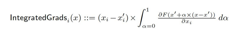
Integrated Gradients
Let's say we have a formal representation of a deep network, F : Rn → [0, 1].
Let x ∈ Rn be the current input and x′ ∈ Rn be the baseline input.
The baseline in image networks might be the black image, whereas it might be the zero embedding vector in text models.
From the baseline x′ to the input x, we compute gradients at all points along the straight-line path (in Rn). By cumulating these gradients, one can generate integrated gradients. Integrated gradients are defined as the path integral of gradients along a direct path from the baseline x′ to the input x.
The two basic assumptions, sensitivity, and implementation invariance, form the basis of this method. Please refer to the original paper to learn more about these axioms.
Gradient SHAP
Shapley values in cooperative game theory are used to compute Gradient SHAP values, which are computed using a gradient approach. Gradient SHAP adds Gaussian noise to each input sample multiple times, then picks a random point on the path between the baseline and the input to determine the gradient of the outputs. As a result, the final SHAP values represent the gradients' expected value. * (inputs - baselines). SHAP values are approximated on the premise that input features are independent and that the explanatory model is linear between the inputs and supplied baselines.
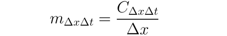
DeepLIFT
It is possible to use DeepLIFT(a back propagation technique) to ascribe input changes based on the differences between inputs and their matching reference (or baseline). DeepLIFT attempts to explain the disparity between the output from reference using the disparity between the inputs from reference. DeepLIFT employs the idea of multipliers to "blame" individual neurons for the difference in outputs. For a given input neuron x with difference-from-reference ∆x, and target neuron t with difference-from-reference ∆t that we wish to compute the contribution to, we define the multiplier m∆x∆t as:
DeepLIFT SHAP
DeepLIFT SHAP is a DeepLIFT extension based on Shapley values established in cooperative game theory. DeepLIFT SHAP computes the DeepLIFT attribution for each input-baseline pair and averages the resultant attributions per input example using a distribution of baselines. DeepLIFT's non-linearity rules help to linearize the network's non-linear functions, and the method's approximation of SHAP values also applies to the linearized network. Input features are likewise presumed to be independent in this method.
Saliency
Calculating input attribution via saliency is a straightforward process that yields the gradient of the output with regard to the input. A first-order Taylor network expansion is used at the input, and the gradients are the coefficients of each feature in the model's linear representation. The absolute value of these coefficients can be used to indicate the relevance of a feature. You can find further information on the saliency approach in the original paper.
Input X Gradient
Input X Gradient is an extension of the saliency approach, taking the gradients of the output with respect to the input and multiplying by the input feature values. One intuition for this approach considers a linear model; the gradients are simply the coefficients of each input, and the product of the input with a coefficient corresponds to the total contribution of the feature to the linear model's output.
Guided Backpropagation and Deconvolution
Gradient computation is performed via guided backpropagation and deconvolution, although backpropagation of ReLU functions is overridden such that only non-negative gradients are backpropagated. While the ReLU function is applied to the input gradients in guided backpropagation, it is directly applied to the output gradients in deconvolution. It is common practice to employ these methods in conjunction with convolutional networks, but they can also be used in other types of neural network architecture.
Guided GradCAM
Guided backpropagation attributions compute the element-wise product of guided GradCAM attributions (guided GradCAM) with upsampled (layer) GradCAM attributions. Attribution computation is done for a given layer and upsampled to fit the input size. Convolutional neural networks are the focus of this technique. However, any layer that can be spatially aligned with the input might be provided. Typically, the last convolutional layer is provided.
Feature Ablation
To compute attribution, a technique known as "feature ablation" employs a perturbation-based method that substitutes a known "baseline" or "reference value" (such as 0) for each input feature before computing the output difference. Grouping and ablating input features is a better alternative to doing so individually, and many different applications can benefit from this. By grouping and ablating segments of an image, we can determine the relative importance of the segment.
Feature Permutation
Feature permutation is a perturbation-based method in which each feature is randomly permuted within a batch, and the change in output (or loss) is computed as a result of this modification. Features can also be grouped together rather than individually in the same way as feature ablation. Note that in contrast to the other algorithms available in Captum, this algorithm is the only one that may provide proper attributions when it is supplied with a batch of multiple input examples. Other algorithms only need a single example as input.
Occlusion
Occlusion is a perturbation-based approach to computing attribution, replacing each contiguous rectangular region with a given baseline/reference and computing the difference in output. For features located in multiple areas (hyperrectangles), the corresponding output differences are averaged to compute the attribution for that feature. Occlusion is most useful in cases such as images, where pixels in a contiguous rectangular region are likely to be highly correlated.
Shapley Value Sampling
The attribution technique Shapley value is based on the cooperative game theory. This technique takes each permutation of the input features and adds them one by one to a specified baseline. The difference in output after adding each feature corresponds to its contribution, and these differences are summed across all permutations to determine attribution.
Lime
One of the most widely used interpretability methods is Lime, which trains an interpretable surrogate model by sampling data points around an input example and using model evaluations at these points to train a simpler interpretable 'surrogate' model, such as a linear model.
KernelSHAP
Kernel SHAP is a technique for calculating Shapley Values that uses the LIME framework. Shapley Values may be obtained more efficiently in the LIME framework by setting the loss function, weighting the kernel, and properly regularizing terms.
Layer Attribution Techniques
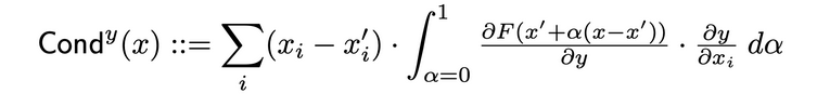
Layer Conductance
Layer Conductance is a method that builds a more comprehensive picture of a neuron's importance by combining the neuron's activation with the partial derivatives of both the neuron with respect to the input and the output with respect to the neuron. Through the hidden neuron, conductance builds upon Integrated Gradients' (IG's) attribution flow. The total conductance of a hidden neuron y is defined as follows in the original paper:
Internal Influence
Using Internal Influence, one can estimate the integral of gradients along the path from a baseline input to the provided input. This technique is similar to applying integrated gradients, which involves integrating the gradient with regard to the layer (rather than the input).
Layer Gradient X Activation
Layer Gradient X Activation is the network's equivalent of the Input X Gradient technique for hidden layers in a network..
It multiplies the activation of the layer element by element with the gradients of the target output with regard to the specified layer.
GradCAM
GradCAM is a convolutional neural network layer attribution technique that is typically applied to the last convolutional layer. GradCAM computes the target output's gradients with respect to the specified layer, averages each output channel (output dimension 2), and multiplies the average gradient for each channel by the layer activations. A ReLU is applied to the output to ensure that only non-negative attributions are returned from the sum of the results across all channels.
Neuron Attribution Techniques
Neuron Conductance
Conductance combines neuron activation with partial derivatives of both the neuron with respect to the input and the output with respect to the neuron to provide a more comprehensive picture of neuron relevance. To determine the conductance of a specific neuron, one examines the flow of IG attribution from each input that passes through that neuron. The following is the original paper's formal definition of conductance of neuron y given input attribution i :

According to this definition, It should be noted that summing the conductance of a neuron (across all input features) is always equal to the conductance of the layer in which that specific neuron is located.
Neuron Gradient
The neuron gradient approach is the equivalence of the saliency method for a single neuron in the network.
It simply computes the gradient of neuron output relative to model input.
This method, like Saliency, may be thought of as doing a first-order Taylor expansion of the neuron's output at the given input, with the gradients corresponding to the coefficients of each feature in the model's linear representation.
Neuron Integrated Gradients
It is possible to estimate the integral of input gradients with respect to a particular neuron throughout the path from a baseline input to the input of interest using a technique called "Neuron Integrated Gradients." Integral gradients are equivalent to this method, assuming the output is just that of the identified neuron. You can find further information on the integrated gradient approach in the original paper here.
Neuron GradientSHAP
Neuron GradientSHAP is the equivalent of GradientSHAP for a specific neuron. Neuron GradientSHAP adds Gaussian noise to each input sample multiple times, chooses a random point along the path between baseline and input, and computes the gradient of the target neuron with respect to each randomly picked point.
The resultant SHAP values are close to the predicted gradient values *. (inputs - baselines).
Neuron DeepLIFT SHAP
Neuron DeepLIFT SHAP is the equivalent of DeepLIFT for a specific neuron. Using distribution of baselines, the DeepLIFT SHAP algorithm computes the Neuron DeepLIFT attribution for each input-baseline pair and averages the resultant attributions per input example.
Noise Tunnel
Noise Tunnel is an attribution technique that can be used in conjunction with other methods. The noise tunnel computes attribution multiple times, adding Gaussian noise to the input each time, and then merges the resulting attributions depending on the chosen type. The following noise tunnel types are supported:
- Smoothgrad: The sampled attributions' mean is returned. Smoothing the specified attribution technique using a Gaussian Kernel is an approximation of this process.
- Smoothgrad Squared: The mean of the squared sample attributions is returned.
- Vargrad: The variance of the sample attributions is returned.
Metrics
Infidelity
Infidelity measures the mean squared error between model explanations in the magnitudes of input perturbations and predictor function's changes to those input perturbtaions. Infidelity is defined as follows:

From well-known attribution techniques such as the integrated gradient, this is a computationally more efficient and extended concept of Sensitivy-n . The latter analyzes the correlations between the sum of the attributions and the differences of the predictor function at its input and a predefined baseline.
Sensitivity
Sensitivity, which is defined as the degree of explanation change to tiny input perturbations using Monte Carlo sampling-based approximation, is measured as follows:

By default, we sample from a subspace of an L-Infinity ball with a default radius to approximate sensitivity. Users can change the ball's radius and the sample function.
Please refer to the algorithm documentation for a complete list of all available algorithms.
Model Interpretation for Pretrained ResNet Model
Bring this project to life
This tutorial shows how to use model interpretability methods on a pre-trained ResNet model with a chosen image, and it visualizes the attributions for each pixel by overlaying them on the image. In this tutorial, we will use the interpretation algorithms Integrated Gradients, GradientShape, Attribution with Layer GradCAM and Occlusion.
Before you start, you must have a Python environment that includes:
- Python version 3.6 or higher
- PyTorch version 1.2 or higher (the latest version is recommended)
- TorchVision version 0
- .6 or higher (the latest version is recommended)
- Captum (the latest version is recommended)
Depending on whether you're using Anaconda or pip virtual environment, the following commands will help you set up Captum:
With conda:
conda install pytorch torchvision captum -c pytorchWith pip:
pip install torch torchvision captumLet us import libraries.
import torch
import torch.nn.functional as F

from PIL import Image

import os
import json
import numpy as np
from matplotlib.colors import LinearSegmentedColormap
import os, sys
import json

import numpy as np
from PIL import Image
import matplotlib.pyplot as plt
from matplotlib.colors import LinearSegmentedColormap

import torchvision
from torchvision import models
from torchvision import transforms

from captum.attr import IntegratedGradients
from captum.attr import GradientShap
from captum.attr import Occlusion
from captum.attr import LayerGradCam
from captum.attr import NoiseTunnel
from captum.attr import visualization as viz
from captum.attr import LayerAttribution
Loads pretrained Resnet model and sets it to eval mode
model = models.resnet18(pretrained=True)
model = model.eval()
The ResNet is trained on the ImageNet data-set. Downloads and reads the list of ImageNet dataset classes/labels in memory.
wget -P $HOME/.torch/models https://s3.amazonaws.com/deep-learning-models/image-models/imagenet_class_index.json
labels_path = os.getenv("HOME") + '/.torch/models/imagenet_class_index.json'
with open(labels_path) as json_data:
    idx_to_labels = json.load(json_data)
Now that we've completed the model, we can download the picture for analysis.
In my case, I chose a cat image.
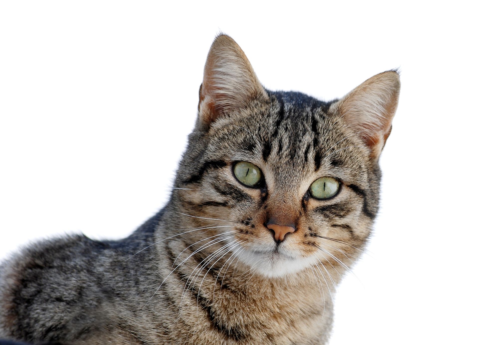
Your image folder must contain the file cat.jpg. As we can see below, Image.open() opens and identifies the given image file and np.asarry() converts it to an array.
test_img = Image.open('path/cat.jpg')
test_img_data = np.asarray(test_img)
plt.imshow(test_img_data)
plt.show()
In the code below, we will define transformers and normalizing functions for the image. To train our ResNet model, we used the ImageNet dataset, which requires images to be of a particular size, with channel data normalized to a specified range of values. transforms.Compose() composes several transforms together and transforms.Normalize() normalizes a tensor image with mean and standard deviation.
# model expectation is 224x224 3-color image
transform = transforms.Compose([
 transforms.Resize(256),
 transforms.CenterCrop(224), #crop the given tensor image at the center
 transforms.ToTensor()
])
# ImageNet normalization
transform_normalize = transforms.Normalize(
     mean=[0.485, 0.456, 0.406],
     std=[0.229, 0.224, 0.225]
 )

img = Image.open('path/cat.jpg')

transformed_img = transform(img)

input = transform_normalize(transformed_img)
#unsqueeze returns a new tensor with a dimension of size one inserted at the #specified position.
input = input.unsqueeze(0)
Now, we will predict the class of the input image. The question that can be asked is, "What does our model feel this image represents?"
#call our model
output = model(input)
## applied softmax() function
output = F.softmax(output, dim=1)
#torch.topk returns the k largest elements of the given input tensor along a given #dimension.K here is 1
prediction_score, pred_label_idx = torch.topk(output, 1)
pred_label_idx.squeeze_()
#convert into a dictionnary of keyvalues pair the predict label, convert it #into a string to get the predicted label
predicted_label = idx_to_labels[str(pred_label_idx.item())][1]
print('Predicted:', predicted_label, '(', prediction_score.squeeze().item(), ')')
output:
Predicted: tabby ( 0.5530276298522949 )The fact that ResNet thinks our image of a cat depicts an actual cat is verified. But what gives the model the impression that this is an image of a cat? To get the solution to that question, we will consult Captum.
Feature Attribution with Integrated Gradients
One of the various feature attribution techniques in Captum is Integrated Gradients. Integrated Gradients awards each input feature a relevance score by estimating the integral of the gradients of the model's output with respect to the inputs.
For our case, we will take a particular component of the output vector - the one that indicates the model's confidence in its selected category - and use integrated gradients to figure out what aspects of the input image contributed to this output. It will allow us to determine which parts of the image were most important in producing this result.
After we have obtained the importance map from Integrated Gradients, we will use the visualization tools captured by Captum to provide a clear and understandable depiction of the importance map.
Integrated gradients will determines the integral of the gradients of the output of the model for the predicted class pred_label_idx with respect to the input image pixels along the path from the black image to our input image.
print('Predicted:', predicted_label, '(', prediction_score.squeeze().item(), ')')
#Create IntegratedGradients object and get attributes
integrated_gradients = IntegratedGradients(model)
#Request the algorithm to assign our output target to
attributions_ig = integrated_gradients.attribute(input, target=pred_label_idx, n_steps=200)
Output:
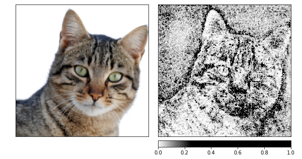
Predicted: tabby ( 0.5530276298522949 )Let's see the image and the attributions that go along with it by overlaying the latter on top of the image. The visualize_image_attr() method that Captum offers provides a set of possibilities for tailoring the presentation of the attribution data to your preferences. Here, we pass in a custom Matplotlib color map(see LinearSegmentedColormap()).
#result visualization with custom colormap
default_cmap = LinearSegmentedColormap.from_list('custom blue',
                                                 [(0, '#ffffff'),
                                                  (0.25, '#000000'),
                                                  (1, '#000000')], N=256)
# use visualize_image_attr helper method for visualization to show the #original image for comparison
_ = viz.visualize_image_attr(np.transpose(attributions_ig.squeeze().cpu().detach().numpy(), (1,2,0)),
                             np.transpose(transformed_img.squeeze().cpu().detach().numpy(), (1,2,0)),
                             method='heat_map',
                             cmap=default_cmap,
                             show_colorbar=True,
                             sign='positive',
                             outlier_perc=1)
Output:
You should be able to notice in the image that we have shown above that the area surrounding the cat in the image is where the Integrated Gradients algorithm gives us the strongest signal.
Let's compute attributions by using Integrated Gradients and then smooth them out over several images that have been produced by a noise tunnel.
The latter modifies the input by adding Gaussian noise with a standard deviation of one, 10 times (nt_samples=10). The smoothgrad_sq approach is used by noise tunnel to make the attributions consistent across all nt_samples of noisy samples.
The value of smoothgrad_sq is the mean of the squared attributions across nt_samples samples. visualize_image_attr_multiple() visualizes attribution for a given image by normalizing the specified sign's attribution values (positive, negative, absolute value, or all) and then displaying them in a matplotlib figure using the selected mode.
noise_tunnel = NoiseTunnel(integrated_gradients)

attributions_ig_nt = noise_tunnel.attribute(input, nt_samples=10, nt_type='smoothgrad_sq', target=pred_label_idx)
_ = viz.visualize_image_attr_multiple(np.transpose(attributions_ig_nt.squeeze().cpu().detach().numpy(), (1,2,0)),
                                      np.transpose(transformed_img.squeeze().cpu().detach().numpy(), (1,2,0)),
                                      ["original_image", "heat_map"],
                                      ["all", "positive"],
                                      cmap=default_cmap,
                                      show_colorbar=True)
Output:
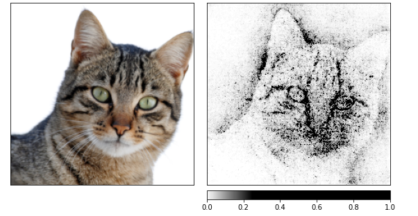
I can see in the images above that the model concentrates on the cat's head.
Let's finish by using GradientShap. GradientShap is a gradient approach that may be used to compute SHAP values, and it is also a fantastic tool for acquiring insight into the global behavior. It is a linear explanation model that explains the model's predictions by using a distribution of reference samples. It determines the expected gradients for an input picked randomly between the input and a baseline.
The baseline is picked at random from the supplied distribution of baselines.
torch.manual_seed(0)
np.random.seed(0)
gradient_shap = GradientShap(model)
# Definition of baseline distribution of images
rand_img_dist = torch.cat([input * 0, input * 1])
attributions_gs = gradient_shap.attribute(input,
n_samples=50,
stdevs=0.0001,
baselines=rand_img_dist,
target=pred_label_idx)
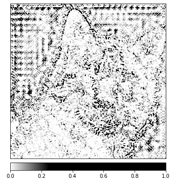
_ = viz.visualize_image_attr_multiple(np.transpose(attributions_gs.squeeze().cpu().detach().numpy(), (1,2,0)),
np.transpose(transformed_img.squeeze().cpu().detach().numpy(), (1,2,0)),
["original_image", "heat_map"],
["all", "absolute_value"],
cmap=default_cmap,
show_colorbar=True)Output:
Layer Attribution with Layer GradCAM
You can relate the activity of hidden layers inside your model to features of your input with the help of the Layer Attribution.
We will apply an algorithm for layer attribution to investigate the activity of one of the convolutional layers included in our model.
GradCAM is responsible for computing the gradients of the target output with respect to the specified layer. These gradients are then averaged for each output channel (dimension 2 of output), and the layer activations are multiplied by the average gradient for each channel.
The results are summed across all channels. Since the activity of convolutional layers often maps spatially to the input, GradCAM attributions are frequently upsampled and used to mask the input. It is worth noting that GradCAM is explicitly developed for convolutional neural networks (convnets). Layer attribution is set up in the same way as input attribution, with the exception that in addition to the model, you must provide a hidden layer inside the model that you want to analyze. Similar to what was discussed before, when we call attribute(), we indicate the target class of interest.
layer_gradcam = LayerGradCam(model, model.layer3[1].conv2)
attributions_lgc = layer_gradcam.attribute(input, target=pred_label_idx)

_ = viz.visualize_image_attr(attributions_lgc[0].cpu().permute(1,2,0).detach().numpy(),
                             sign="all",
                             title="Layer 3 Block 1 Conv 2")
To make a more accurate comparison between the input image and this attribution data, we will upsample it with the help of the function interpolate(), located in the LayerAttribution base class.
upsamp_attr_lgc = LayerAttribution.interpolate(attributions_lgc, input.shape[2:])

print(attributions_lgc.shape)
print(upsamp_attr_lgc.shape)
print(input.shape)

_ = viz.visualize_image_attr_multiple(upsamp_attr_lgc[0].cpu().permute(1,2,0).detach().numpy(),
                                      transformed_img.permute(1,2,0).numpy(),
                                      ["original_image","blended_heat_map","masked_image"],
                                      ["all","positive","positive"],
                                      show_colorbar=True,
                                      titles=["Original", "Positive Attribution", "Masked"],
                                      fig_size=(18, 6))
Output:
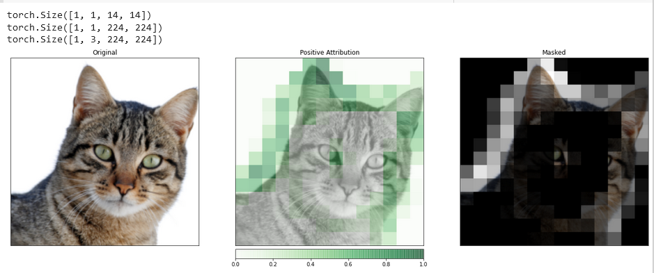
Visualizations such as this one have the potential to provide you with unique insights into how your hidden layers respond to the input you provide.
Feature Attribution with Occlusion
Methods based on gradients help understand the model in terms of directly computing the changes in the output with regard to the input.
The technique known as perturbation-based attribution takes a more direct approach to this problem by making modifications to the input to quantify the impact such changes have on the output. One such strategy is called occlusion.
It entails swapping out pieces of the input image and analyzing how this change affects the signal produced on the output.
In the following, we will configure the occlusion attribution. Like the configuration of a convolutional neural network, you can choose the target region's size and a stride length, which determines the spacing of individual measurements.
We will use the visualize_image_attr_multiple() function to view the results of our Occlusion attribution. This function will display heat maps of both positive and negative attribution per region and mask the original image with the positive attribution regions.
The masking provides a very illuminating look at the regions of our cat photo that the model identified as most "cat-like."
occlusion = Occlusion(model)

attributions_occ = occlusion.attribute(input,
                                       target=pred_label_idx,
                                       strides=(3, 8, 8),
                                       sliding_window_shapes=(3,15, 15),
                                       baselines=0)


_ = viz.visualize_image_attr_multiple(np.transpose(attributions_occ.squeeze().cpu().detach().numpy(), (1,2,0)),
                                      np.transpose(transformed_img.squeeze().cpu().detach().numpy(), (1,2,0)),
                                      ["original_image", "heat_map", "heat_map", "masked_image"],
                                      ["all", "positive", "negative", "positive"],
                                      show_colorbar=True,
                                      titles=["Original", "Positive Attribution", "Negative Attribution", "Masked"],
                                      fig_size=(18, 6)
                                     )
Output:
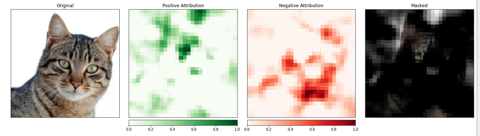
The portion of the image containing the cat seems to be given a higher level of importance.
Conclusion
Captum is a model interpretability library for PyTorch that is versatile and simple. It offers state-of-the-art techniques for understanding how specific neurons and layers impact predictions.
It has three main types of attribution techniques: Primary Attribution Techniques, Layer Attribution Techniques, and Neuron Attribution Techniques.
References
https://pytorch.org/tutorials/beginner/introyt/captumyt.html
https://captum.ai/docs/algorithms
https://captum.ai/docs/introduction.html
https://gilberttanner.com/blog/interpreting-pytorch-models-with-captum/
https://arxiv.org/pdf/1805.12233.pdf
https://arxiv.org/pdf/1704.02685.pdf


