The hyperparameter optimization problem has been solved in many different ways for classical machine learning algorithms. Some examples include the use of grid search, random search, Bayesian optimization, meta-learning, and so on. But when considering deep learning architectures, the problem becomes much harder to deal with. In this article we will cover the problem of neural architecture search and the current state of the art. This article assumes a basic knowledge of different neural networks and deep learning architectures.

This is Part 1 of a series which will take you through what the problem of neural architecture search (NAS) is, and how to implement various interesting approaches for NAS using Keras. In this part we'll cover topics like the controller (RNNs), REINFORCE gradient, genetic algorithms, controlling the search space, and designing the search strategy. This will include a literature review of state of the art papers in the field.

Introduction

Deep learning engineers are expected to have an intuitive understanding of what architecture might work best for what situation, but this is rarely the case. The possible architectures one can create are endless. Think about all of the convolutional backbones trained on ImageNet that we use for transfer learning. Take for example ResNet, which has variants with 50, 100, and 150 layers. There are many ways in which you can tweak these architectures–adding an extra skip connection, removing a convolutional block, etc.

The aim of neural architecture search is to automate the process of finding the best model architecture, given a dataset.

The first paper to make this a popular area of research came from Zoph et al. (2016). The idea was to use a controller (a recurrent neural network) to generate an architecture, train it, note its accuracy, train the controller according to the gradient calculated, and finally determine which architecture performed the best. In other words, it would evaluate all (or at least, many) possible architectures and find the one that gave the best validation accuracy.

This exploration of the entire search space was only meant for those with a huge amount of computational resources. Thankfully, over time, several faster and more efficient ways of performing the task of neural architecture search have been developed.

The Basics of Neural Architecture Search

To understand the major approaches that have been applied to this task we will require some cross-domain knowledge of deep learning, optimization, and computer sciences. The approaches people have taken to solve this problem range from reinforcement learning to evolutionary algorithms.

The earlier solutions to neural architecture search can be visualized as a multi-step loop, which goes something like this:

In other words:

1. Use a controller to generate an architecture
2. Train the generated architecture for a few epochs
3. Evaluate the generated architecture
4. Understand how well said architecture is performing
5. Update your controller accordingly
6. Repeat.

This broad overview gives us an idea of the problem we’re trying to solve but leaves several questions unanswered, like:

1. What is the best way to design the controller?
2. How do we optimize for better architecture generation?
3. How do we reduce our search space efficiently?

To answer these questions, we should first discuss some of the basic theory.

The Controller: Recurrent Networks

Most of you reading this article are probably already aware of what RNNs are, but we will still touch up on the basic concepts for the sake of completeness. Recurrent Neural Networks take in sequential inputs and predict the next element in the sequence depending on the data they’re trained on. Vanilla recurrent networks would, based on the input provided, process their previous hidden state and output the next hidden state and a sequential prediction. This prediction is compared with the ground truth values to update weights using backpropagation.

We also know that RNNs are susceptible to vanishing and exploding gradients. To fix this problem, LSTMs came into being. LSTMs use different gates to manage the amount of importance given to each previous element in the sequence. There are also bi-directional variants of LSTMs which learn the sequential dependence of different elements from left to right, as well as right to left.

In the context of neural architecture search, recurrent networks in one form or another will come in handy as they can serve as controllers which create sequential outputs. These sequential outputs will be decoded to create neural network architectures that we will train and test iteratively to move towards better architecture modelling.

REINFORCE Gradient

A reinforcement learning flow looks something like this. Given an environment, the current state and the possible set of actions:

1. Our agent takes an action according to a policy
2. The environment is manipulated and a new state is created
3. Based on the reward function, our agent updates its policy
4. Repeat with the new state and updated policy

"Policy gradients" refer to the different ways this policy can be updated. REINFORCE is a policy gradient algorithm which was initially used on NAS to optimize the process of architecture search by controllers. The REINFORCE policy gradient tries to optimize an objective function in a way that maximizes the agent’s total rewards by maximizing the product of log-likelihood per search step with the reward at each step. Reward can be some function of the validation accuracy of each architecture created by the controller.

For neural architecture search we will find that our controllers can be optimized to create better architectures by using the REINFORCE gradient. Here, actions would be the possible layers or connections in your architecture, and policy would be the softmax distribution of these layers per controller step.

Genetic Algorithms

The same optimization process can be done using genetic algorithms, a class of algorithms which aim to replicate how populations evolve in nature to optimize functions. The overall workflow looks something like this: given an initial population of solutions...

1. Evaluate the fitness of each solution. This is designed specifically for your optimization problem. Depending on what your objective is, you’d have to find an appropriate fitness function.
2. Select the population fittest to create offspring. There are several selection schemes that we can use to pick the parents–ranked selection where we pick the fittest from the sorted fitness values, roulette wheel selection where we account for chance, tournament selection where we allow for the winners of a tournament to be selected for further evolution, etc.
3. Create offspring and mutations. In digital evolution the offspring do not need to have only two parents. The genes in each phenotype or the different variables of each solution can be mixed and matched in several ways to create offspring. The future generation is also created by a certain section of the population that mutates in various ways.
4. Repeat the process with the new generation of solutions.

There are several ways of performing each of these steps. Genetic algorithms have become more complex, accounting for lifespan, multi-objective optimization, elitism, diversity, curiosity, archiving previous generations, etc.

Another concept that is important to know with respect to evolutionary algorithms is that of Pareto Optimality. A Pareto front is the state of allocation of resources in a manner that makes it impossible to deviate from the state in a way that will benefit one party without harming the other. This concept comes in handy when trying to balance multi-objective trade-offs, like in neural architecture search when finding the optimal solution must balance both accuracy and efficiency for scalability purposes.

Neural Architecture Search

In the 2017 paper by Zoph et al., the methodology followed was to generate the layer hyperparameters (for example, a convolutional layer would require stride, kernel size, number of kernels, whether or not it has a skip connection, etc.) sequentially. These hyperparameters are what we call a search space. The generated architectures were trained on the CIFAR-10 dataset for a certain number of epochs. The reward function used was the maximum validation accuracy found in the last 5 epochs cubed, and the controller was updated using the REINFORCE policy gradient.

This, at least for several initial epochs, feels like mindless attempts at creating architectures.

Controlling the Search Space

NAS algorithms design a specific search space and hunt through the search space for better architectures. The search space for convolutional network design in the paper mentioned above can be seen in the diagram below.

The algorithm would stop if the number of layers exceeded a maximum value. They also added skip connections, batch normalization and ReLU activations to their search space in their later experiments. Similarly, they create RNN architectures by creating different recurrent cell architectures using the search space shown below.

The biggest drawback of the approach mentioned above was the time it took to navigate through the search space before coming up with a definite solution. They used 800 GPUs for 28 days to navigate through the entire search space before coming up with the best architecture. There was clearly a need for a way to design controllers that could navigate the search space more intelligently.

To this end, Zoph et al. (2017) attempted to tackle this problem by breaking it down into two steps:

1. Designing cells for convolutional blocks
2. Stacking a certain number of blocks to create architectures

They used an expanded search space that included convolutions, pooling, and depth-separable convolutions of various kernel sizes, to first create:

1. A normal cell. Convolutional cells that return a feature map of the same size as the input
2. A reduction cell. Convolutional cells that return a feature map of half the width and height of the initial input

Novel approaches to constraining the search space have also been developed, like by Ghiasi et al. (2019) who adopt the MobileNet framework and tune for better Feature Pyramid Networks, and then stack the FPN architectures for a set number of times to generate the final architectures. Chen et al. (2019) do the same for backbone architectures of different object detection algorithms. As pointed out by Elsken et al. (2019), these approaches also bring up the problem of designing macro-architectures, considering how many cell blocks need to be stacked and how they are connected with each other.

Designing the Search Strategy

Most of the work that has gone into neural architecture search has been innovations for this part of the problem: finding out which optimization methods work best, and how they can be changed or tweaked to make the search process churn out better results faster and with consistent stability. There have been several approaches attempted, including Bayesian optimization, reinforcement learning, neuroevolution, network morphing, and game theory. We will look at all of these approaches one by one.

1. Bayesian Optimization

Bayesian optimization approaches saw a lot of success in the early work for neural architecture search. Bayesian optimization works by optimizing an acquisition function for a surrogate model to guide the selection of the next evaluation point. The steps (as mentioned in this article) are as follows:

Initialization
      - Place a Gaussian process prior on f
      - Observe f at n_0 points according to an initial space-filling
        experimental design
      - Set n to n_0

While n ≤ N do
      - Update the posterior probability distribution of f using all
	available data
      - Identify the maximiser x_n of the acquisition function over the valid
        input domain choices for parameters, where the acquisition function is
        calculated using the current posterior distribution
      - Observe y_n = f(x_n)
      - Increment n
End while

Return either the point evaluated with the largest f(x) or the point
with the largest posterior mean.

Kandasamy et al. (2018) created NASBOT, a Gaussian process-based approach for neural architecture search for multi-layer perceptrons and convolutional networks. They calculate a distance metric through an optimal transport program to navigate the search space. Zhou et al. (2019) propose BayesNAS which applies classic Bayes Learning for one shot architecture search (there's more about one shot architecture search in the final section).

2. Reinforcement Learning

Reinforcement learning has been used successfully in driving the search process for better architectures. As discussed earlier, the initial approaches to NAS were dominated by the use of the REINFORCE gradient as the search strategy (e.g. Zoph et al. (2016) and Pham et al. (2018)). Other approaches like Proximal Policy Optimization and Q Learning are applied for the same problem by Zoph et al. (2018) and Baker et al. (2016), respectively. You can learn more about PPO algorithms here and about Q Learning here.

The ability to navigate the search space efficiently in order to save precious computational and memory resources is typically the major bottleneck in an NAS algorithm. Often, the models built with the sole objective of a high validation accuracy end up being high in complexity–meaning a greater number of parameters, more memory required, and higher inference times. An important contribution with reinforcement learning to combat these issues was made by Hsu et al. (2018), where they proposed MONAS: Multi-Objective Neural Architecture Search using reinforcement learning. MONAS attempts to optimize for scalability by building a novel optimization objective; one that accounts for not just good validation accuracy, but also minimal power consumption.

A mixed reward function is defined:

R = α∗Accuracy − (1−α)∗Energy

Another interesting effort to reduce the inference latency is attempted by Guo et al. (2018), who try to create a search method in a way that would mimic how humans design architectures: by training an agent to learn the topology of human-designed search network structures.

Agents intelligently navigate the search space to build architectures that are guided by human-designed topologies using inverse reinforcement learning (IRL). IRL is a paradigm relying on Markov Decision Processes (MDPs), where the goal of the apprentice agent is to find a reward function from the expert's demonstrations that could explain the expert's behavior. Reinforcement learning tries to maximize the reward by optimizing its policy, whereas in inverse reinforcement learning we are given an expert policy that we try to explain by finding the optimal reward function.

They propose a mirror stimuli function inspired by biological cognition theory to extract the abstract topological knowledge of an expert human-designed network (ResNet). They answer two major questions in their work:

1. How to encode topologies in a way that the agent would understand?
2. How to use this information to guide our search process?

Let's take a look at how they answer these two questions.

How to encode topologies in a way that the agent would understand?

The authors use the hyperparameters of the two previous layers of the network (kernel size, operation type, and indexes) to encode what they call the "state feature code." They encode these feature codes into embeddings using feature counts as described in the formula below.

Where φ is the state feature function, s is the state of the environment, t represents iterations (since each state at a given time is an architecture created by our agent) that varies from 1 to T (can be an upper bound or calculated according to some convergence criteria, it isn't clear in the paper); γ denotes a discounted scalar which takes care of time dependencies.

How to use this information to guide our search process?

Here they are faced with the classic exploration-exploitation trade off, where the algorithm needs to create architectures topologically, similar to the expert networks, while also efficiently exploring the search space. Policy imitation would lead our network to raise strong priors and inhibit the search process. To avoid this, they design a mirror stimuli function:

The problem of optimization becomes similar to finding a time-step reward function r(st) =wT·φ(st). This is done with a match function as proposed by Andrew Ng and Pieter Abbeel. The final reward function is calculated as follows:

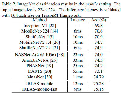
They apply Q Learning using a normalized version of the reward shown above to guide their search. IRLAS is able to achieve state of the art results on ImageNet, and in a mobile setting.

3. Neuroevolution

Floreano et al. (2008) claim that gradient-based methods outperform evolutionary methods for the optimization of neural network weights, and that evolutionary approaches should only be used to optimize the architecture itself. Besides deciding on the right genetic evolution parameters like mutation rate, death rate, etc., there's also the need to evaluate how exactly the topologies of neural networks are represented in the genotypes we use for digital evolution.

This representation can be:

1. Direct, where each property of our networks to be optimized will be directly linked to a gene
2. Indirect, where the connection between genotypes and phenotypes is not a one-to-one mapping but a set of rules that describe how to go about creating an individual

Stanley et al. (2002) proposed NEAT, which uses a direct encoding strategy to represent different nodes and connections in a neural network. Their genotype representation includes node genes and connection genes, each of which directly describe how different nodes in your network are connected, if they are active, etc. Mutation in NEAT involves modifying a connection or adding a new connection. The paper also addresses the competing conventions issue–the possibility of creating worse networks due to blind crossovers.

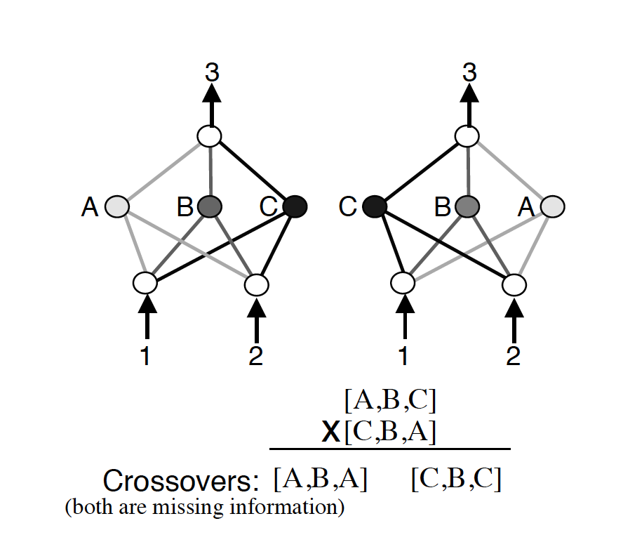
NEAT tackles this issue through the use of historical markings (shown above). By marking new evolutions with a historical number, when it comes time to crossover two individuals, this can be done with a much lower chance of creating individuals that are non-functional. Another measure taken is the use of speciation, or grouping different generated architectures according to their topologies. Each new architecture then only has to compete with its own "species".

On the other hand, Compositional Pattern Producing Networks (CPPNs) provide a powerful indirect encoding that can be evolved with NEAT for better results. You can learn more about CPPNs here, and find an implementation and visualizations in an article by David Ha here. Another variation of NEAT known as HyperNEAT also uses CPPNs for encoding, and evolves with the NEAT algorithm. Irwin-Harris et al. (2019) propose an indirect encoding method which uses directed acyclic graphs to encode different neural network architectures for evolution.

Stanley et al. (2019) highlight the ability to account for diversity in genetic algorithms, which increases the chance of finding novel architectures and also allows for massively parallel exploration. Accounting for diversity is also important for problems with multiple local optima, and to avoid genetic drift. To aid diversity, much of the earlier work tried to expand the genetic space based on the idea that if the evolution process was directed to go away from the locally optimal solutions, it would help exploration and encourage novelty. They include niching methods like crowding, in which a new individual replaces the one most genetically similar to it, and fitness-sharing, in which individuals are clustered by genetic distance and are punished by how many members are in their cluster.

Although sometimes effective, these methods also fail since such solutions often aren't optimal and have a low fitness. To address this issue, Stanton et al. (2018) incorporate curiosity in a reinforcement learning algorithm for better exploration. Gravina et al. (2016) introduce the element of surprise generation to encourage diversity. Other methods to incorporate diversity in evolutionary algorithms can be found in this paper.

As pointed out by Elsken et al. (2018), an advantage of using evolutionary algorithms over other optimization methods is the flexibility they provide in the design of a performance function. The fitness functions can range from extremely simple to very complex, and give us a lot of room to experiment when compared to error rates or log-likelihood functions. Elsken et al. (2019) solve for scalability, high accuracy, and low resource consumption by proposing LEMONADE. This is an evolutionary algorithm for multi-objective architecture search that allows approximating the entire Pareto front of architectures under multiple objectives, such as predictive performance and number of parameters, in a single run of the method.

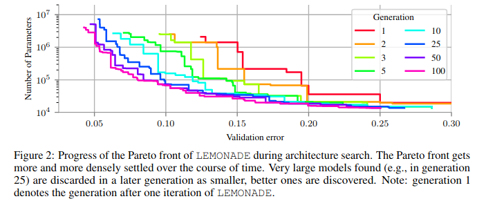
To reduce the computational resources to run a neuroevolution method itself, they add a Lamarckian Inheritance mechanism for LEMONADE that generates child networks which draw from their parent networks using network morphing operations.

4. Network Morphing

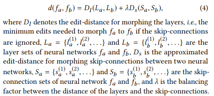
Jin et al. (2019) built AutoKeras, an open source NAS engine that functions a bit like AutoML. Their framework utilizes Bayesian optimization to guide network morphism. To guide the morphing operations through the search space, an edit distance-based kernel is constructed (since architecture representations evade a Euclidean representation). Edit distance refers to how many morphing operations are required to transform one network into another, and the kernel function is defined as follows:

where d denotes the edit distance between architectures f_a and f_b, and p is the mapping function that maps the edit distance to the new space. This new space is based on embedding the original metric into a new one using the Bourgain theorem. The edit distance is approximated for this NP hard problem as follows.

They apply Bayesian Optimization for network morphing by designing a novel acquisition function for a tree-structured space. They not only morph the leaves of the tree structure but also the inner nodes, allowing them to morph into smaller architectures as well and avoid iteratively building bigger and more complex architectures. A* search and simulated annealing are proposed to balance exploration and exploitation. They achieve impressive results on classification tasks.

Kwasigroch et al. (2019) propose a network morphing approach for neural architecture search using evolutionary algorithms and the hill climbing algorithm for the problem of detecting malignant melanoma. The hill climbing strategy works by iteratively perturbing an initial solution to create new solutions until the best one is found. The hill climbing strategy applied to NAS with evolutionary algorithm-inspired morphing operations is visualized below.

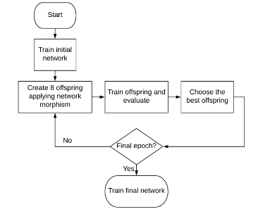
The structure of the initial network is four blocks of [Conv, BatchNorm, ReLU, MaxPool] followed by a final block of [Conv, BatchNorm, ReLU, Sigmoid]. The convolution layer contains 128 filters of 3x3 kernels with a stride 1, whereas the max pooling layer contains 2x2 windows with a stride 2. The networks are trained with a warm restart stochastic gradient descent with a decaying learning rate.

5. Game Theory

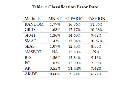
Liu et al. (2019) proposed DARTS, a differentiable architecture search method that leverages game theoretic concepts for the optimization of neural architectures. They pose the architecture search problem as bilevel optimization, where one optimization problem is embedded in another. Nayman et al. (2019) propose an architecture search method that bases itself on the decision science concept of minimizing regrets. They reformulate the DARTS approach in a way that allows for direct optimization of architecture weights by leveraging PEA theory (Prediction with Expert Advice) and propose XNAS. The PEA framework uses a forecaster/decision maker which tries to sequentially make decisions, in our case building neural architectures, using expert advice.

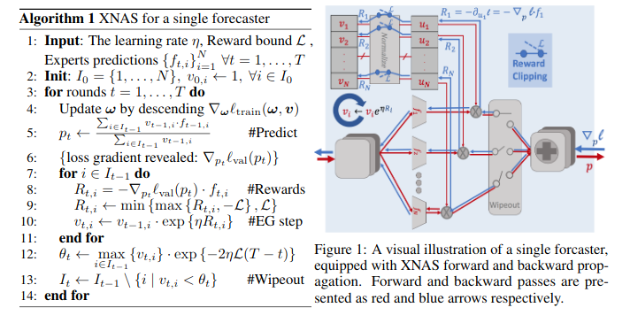
These expert networks make predictions at each time step, which direct the forecaster's decisions. They use the exponentiated-gradient rule for optimization. The optimizer then removes the weak experts and effectively reassigns weights to the remaining ones.

Model Compression

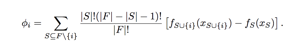
While not exactly in the domain of architecture search, an important consideration in designing neural architectures is that of model compression. Several approaches have been adapted over time: quantization, pruning, knowledge distillation, etc. It is worth mentioning the work of Stier et al. (2019), who propose a game theoretic approach based on Shapley Values to create efficient network topologies. Shapley values are the predominant solution to a game theory problem: how best to divvy up the collective payoff in a coalition of players with different skill sets? For a subset of players, the Shapley value can be thought of as the expected marginal contribution of the player in the collective payoff. It is calculated as shown below.

An explanation of how Shapley values and marginal payoffs work can be found here.

The players can be seen as the structural components of a network. For example, each neuron in a single hidden layer network would function as a player in this coalition game. For the payoff function, several different possible choices exist, like training loss, validation accuracy, etc. In this work, the cross-entropy accuracy is used as the payoff function due to its bounded nature. They subtract a baseline (regression accuracy) from the evaluation accuracy to obtain the payoff. The Shapley values are approximated by random sampling, and are used to finally prune the model to reduce the number of players depending on which ones have the lowest Shapley values.

Performance Estimation Strategy

Elsken et al. (2019) mention the need for speeding up performance estimation of NAS methods. A simple approach to measuring performance of generated architectures could be measuring the validation accuracy. But for a large search space, big dataset, and several-layer deep networks, this becomes a time consuming and computationally heavy task. To avoid this, they suggest several strategies like using low fidelity estimates obtained by training for fewer epochs, or on a small subset of data as is done by Real et al. (2019). This approach can work if we can be sure that the relative ranking of architectures does not change due to the low fidelity evaluations. But recent research has shown this not to be the case.

Another strategy is based on extrapolating from learning curves. Architectures that are predicted to perform poorly from the learning curve in the initial few epochs can be terminated to speed up the search process. Liu et al. (2018), on the other hand, don't use learning curves but suggest training a surrogate model to predict the performance of an architecture based on properties that are extrapolated from other novel architectures.  

One-shot architecture search, popularized by Pham et al. (2018), are NAS methods which attempt to train one super-architecture which subsumes all the other architectures in the search space. This is done by sharing parameters between all the networks that are created by the search space navigation strategy. One-shot methods allow for fast evaluation since the weights of the super-graph can be inherited to evaluate the various different architectures with training them. While one-shot NAS has reduced the computational resources required for neural architecture search, it is unclear how the inheritance of weights from the super-graph affects the performance of the sub-graphs and the kind of biases it introduces into architectures.

Summary

In this article we reviewed the problem of neural architecture search by dividing it into three areas of active research. We looked at how the search space is designed, how the search strategy is designed (either with Bayesian optimization, reinforcement learning, evolutionary algorithms, network morphism, or game theory), and finally we looked at different ways to speed up architecture performance estimation (namely low fidelity estimations, learning curve extrapolation, and one-shot learning).

We skipped much of the literature about compression of neural networks using pruning, quantization, and knowledge distillation, as this belongs more to a discussion of how to build efficient architectures given a parent architecture. Another long-form post could easily be devoted to this topic alone. I still felt the need to mention this topic briefly due to the increasing attention these techniques are getting currently, and the road they pave to democratizing machine learning.

I hope you found this article useful.

In the next part of this series, we will start looking at how to implement NAS for Multilayer Perceptrons in order to see how the core concepts discussed here work in action.