How To Implement Support Vector Machine With Scikit-Learn

In this tutorial we'll cover:

1. An introduction to the support vector machine algorithm
2. Implementing SVM using Python and Sklearn

So, let's get started!

Introduction to Support Vector Machine

Support Vector Machine (SVM) is a supervised machine learning algorithm that can be used for both classification and regression problems. SVM performs very well with even a limited amount of data.

In this post we'll learn about support vector machine for classification specifically. Let's first take a look at some of the general use cases of the support vector machine algorithm.

Use Cases

Classification of Disease: For example, if we have data about patients with a disease like diabetes, we can predict whether a new patient is likely to have diabetes or not.

Classification of Text: First we need to transform the text into a vector representation. Then we can apply the support vector machine algorithm to the encoded text in order to assign it to a specific class.

Classification of Images: Images are converted to a vector containing the pixel values, then SVM assigns a class label.

Let's now understand some of the key terms related to SVM.

Key Terms

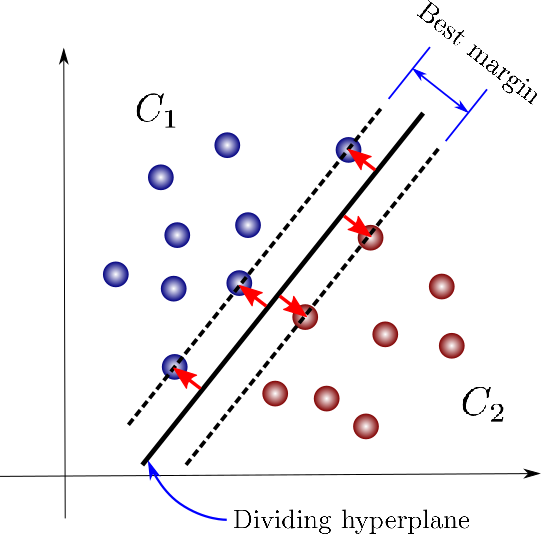
Support Vector: Support vectors are the data points that are closer to a hyperplane, as shown in the image above. Using the support vectors, the algorithm maximizes the margin, or separation, between classes. If the support vectors are changed, the position of the hyperplane will also change.

Hyperplane: A hyperplane in two dimensions is simply a line that best separates the data. This line is the decision boundary between the classes, as shown in the image above. For a three-dimensional data distribution the hyperplane would be a two dimensional surface, not a line.

Margin: This is the distance between each of the support vectors, as shown above. The algorithm aims to maximize the margin. The problem of finding the maximum margin (and hence, the best hyperplane) is an optimization problem, and can be solved by optimization techniques.

Kernel: The kernel is a type of function which is applied to the data points in order to map the original non-linear data points into a high dimensional space where they are separable. In many cases there will not be a linear decision boundary, which means that no single straight line will separates both classes. Kernels address this issue. There are many kinds of kernel functions available. an RBF (radial basis function) kernel is commonly used for classification problems.

Having understood these key terms, let's dive into an exploration of the data.

Exploratory Data Analysis

First we'll import the required libraries. We're importing numpy, pandas and matplotlib. Apart form that we also need to import SVM from sklearn.svm.

We'll also be using train_test_split from sklearn.model_selection, and accuracy_score from sklearn.metrics. We'll use matplotlib.pyplot for visualization.

import numpy as np
import pandas as pd
from sklearn.model_selection import train_test_split
from sklearn.svm import SVC
from sklearn.metrics import accuracy_score
import matplotlib.pyplot as plt

Once the libraries are imported we need to read the data from the CSV file to a Pandas data frame. Let's check the first 10 rows of data.

The data is a collection of data for medical patients checked for potential diabetes. For simplicity we are considering two features age and glucose level and one target variable which is binary. The value of 1 indicates diabetes and 0 indicates no diabetes.

df = pd.read_csv('SVM-Classification-Data.csv')
df.head()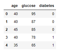

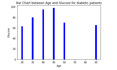
To get more idea about the data we have plotted a bar chart of data as shown below. A bar chart is a chart that presents categorical data with rectangular bars with heights representing the values that they have. The bar charts can be plotted vertically or horizontally.

The below graph is a vertical chart between Age and Glucose column.

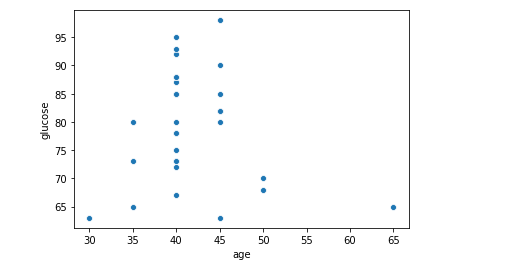
To get a better idea of outliers we may like to look at a scatter plot as well. Below is scatter plot of the features present in the data.

After exploring the data , we may like to do some of the data pre processing tasks as below.

Data Pre-Processing:

Before feeding the data to the support vector classification model, we need to do some pre-processing.

Here we are going to create two variables x and y. x represents features for the model and y represents the label for the model. We will create the x and y variables by taking them from the dataset and using the train_test_split function of sklearn to split the data into training and test sets.

x = df.drop('diabetes',axis=1)
y = df['diabetes']
x_train, x_test, y_train, y_test = train_test_split(x, y, test_size=0.25, random_state=42)

Note that the test size of 0.25 indicates we’ve used 25% of the data for testing. random_state ensures reproducibility. For the output of train_test_split, we get x_train, x_test, y_train, and y_test values. We are going to use x_train and y_train to train the model and then we will use x_test and y_test together to test the model.

After the data pre processing is done its time now to define and fit the model.

Define and Fit Model

We'll create a model variable and instantiate the SVC class. After this we will be training the model, but before that let us discuss some of the important parameters of the support vector classifier model, listed below.

Kernel: kernel refers to the class of algorithms for pattern analysis. This is an string parameter and is optional. The default value is RBF. The popular possible values are ‘linear’, ‘poly’, ‘rbf’, ‘sigmoid’, ‘precomputed’.

Linear Kernel is one of the most commonly used kernels. This is used when the data is Linearly separable means data can be separated using a single Line.

RBF kernel is used when the data is not linearly separable. The RBF kernel of Support Vector Machine creates a non-linear combinations of given features and transforms the given data samples to a higher dimensional feature space where we can use a linear decision boundary to separate the classes.

Regularization C: C is a regularization parameter. The regularization is inversely proportional to C. It must be positive.

Degree: Degree is the degree of the polynomial kernel function. It is ignored by all other kernels like linear.

Verbose: This enables verbose output. Verbose is a general programming term for produce most of logging output. Verbose means asking the program to tell everything about what it is doing all the time.

Random_State: random_state is the seed used by the random number generator. This is used to ensure reproducibility. In other words, to obtain a deterministic behavior during fitting, random_state has to be fixed.

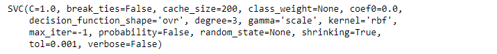
SupportVectorClassModel = SVC()
SupportVectorClassModel.fit(x_train,y_train)

After we defined the model above we need to train the model using the data given. For this we are using the fit() method as shown above. This method is passed two parameter, which is our data of interest (in this case, the age and glucose as well as diebetes training part of the dataset).

Once the model is trained properly it will output the SVC instance as shown in the output of the cell below.

Model training completion will automatically lead you to try out some predictions.

Predicting Using Model

Once the model is trained, it’s ready to make predictions. We can use the predict method on the model and pass x_test as a parameter to get the output as y_pred.

Notice that the prediction output is an array of real numbers corresponding to the input array.

y_pred = SupportVectorClassModel.predict(x_test)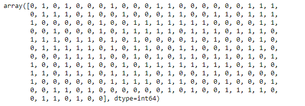

Once the prediction is done , naturally we would like to test the accuracy of the model.

Evaluating the Model

Now this is the time to check to see how well our model is performing on the test data. For this, we evaluate our model by finding the accuracy produced by the model.

We are going to use accuracy_score function and we will pass two parameters y_test and y_pred to this function.

accuracy = accuracy_score(y_test,y_pred)*100
99.19678714859438

As you can see above the accuracy measured for this model is around 99.19%.

End Notes

In this tutorial we learned what is a Support Vector Machine Algorithm and its use cases. We also discussed various exploratory data analysis graphs like bar plot and scatter plot for this problem.

Finally we implemented the Support Vector Classification Algorithm and printed the prediction.

I hope you liked the article and you may like to use it in your project in future if required.

Happy Learning!