Visual Question Answering: a Survey

We've seen a lot of advancements in the last few years in many subdomains of machine learning. Computer vision tasks like object detection and image segmentation, as well as NLP tasks like entity recognition, language generation, and question answering, are now being solved by neural networks and approached much differently, with more speed and higher accuracy.

A task that has grasped the attention of the AI community recently is that of visual question answering. This article will explore the problem of visual question answering, different approaches to solve it, associated challenges, datasets, and evaluation methods.

Introduction

Visual question answering systems attempt to correctly answer questions in natural language regarding an image input. The broader idea of this problem is to design systems that can understand the contents of an image similar to how humans do, and communicate effectively about that image in natural language. This is a challenging task since it requires image-based models and natural language models to interact with and complement each other.

The problem has widely been accepted as AI-complete, i.e. one that confronts the Artificial General Intelligence problem, namely making computers as intelligent as people. In fact, the problem has also been suggested to be used as a Visual Turing Test by Geman et al. (2015).

To give you an idea of the subproblems the task of visual question answering entails:

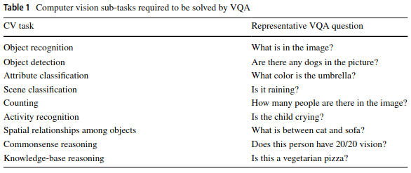
Solutions to these problems involve four major steps:

• Image featurization - converting images into their feature representations for further processing.
• Question featurization - converting natural language questions into their embeddings for further processing.
• Joint feature representation - ways of combining image features and the question features to enhance algorithmic understanding.
• Answer generation - utilizing the joint features to understand the input image and the question asked, to finally generate the correct answer.

Each phase in this pipeline has been approached in several ways. We will look through the primary ones in this article.

Image Featurization

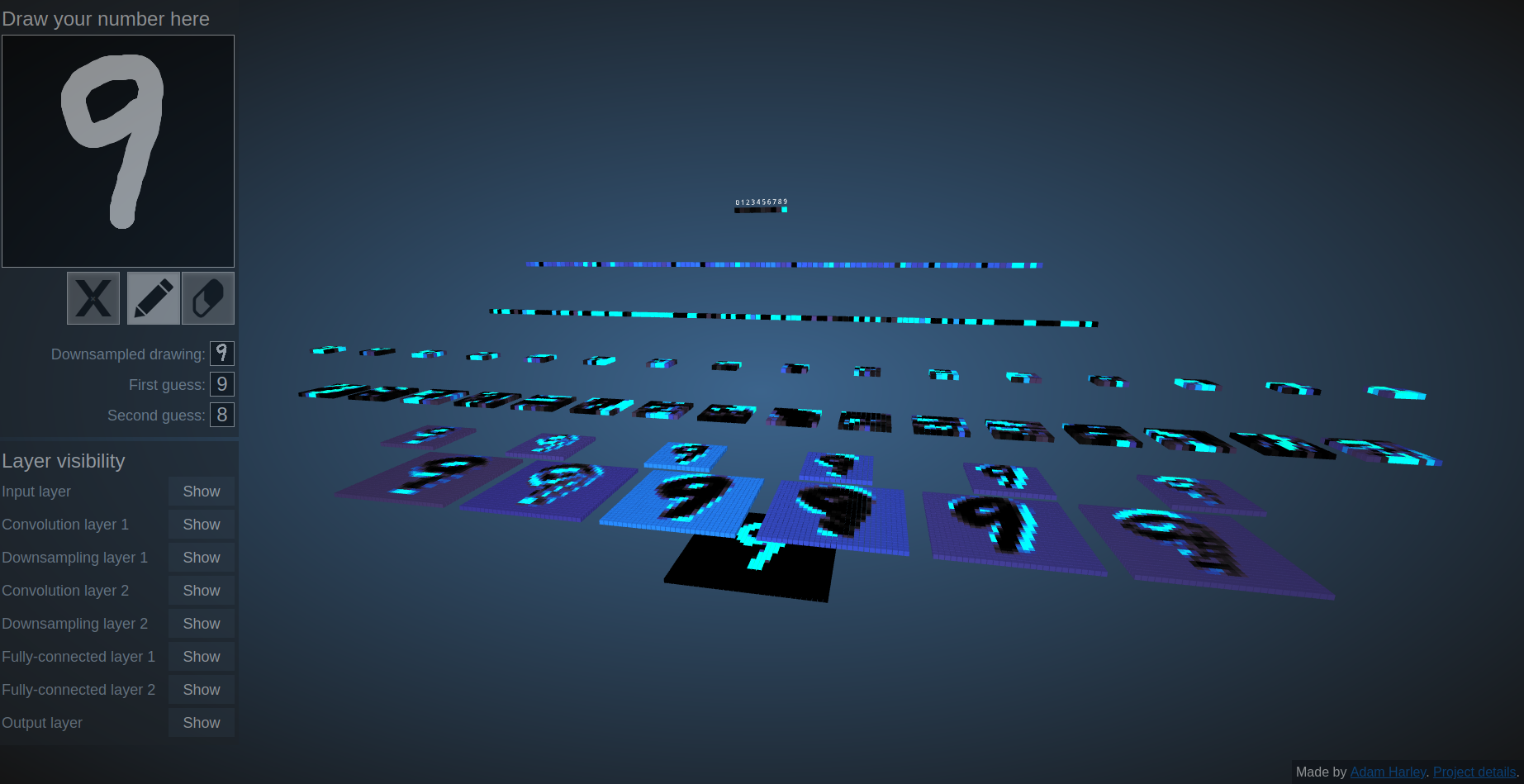
Convolutional neural networks have become the gold-standard for pattern recognition in images. After an input image is passed through a convolutional network, it gets transformed into an abstract feature representation. Each filter in a CNN layer captures different kinds of patterns, such as edges, vertices, contours, curves, and symmetries. This concept is explained very well in this article, which discusses equivariance in neural networks and how activation maps look for different kinds of detectors.

Check out the 3-D visualization tool for a CNN-based network trained on MNIST data for hand-written digit recognition here.

CNNs have evolved into deeper and more complicated architectures which are widely used for downstream tasks like classification, object detection, and image segmentation. Some such networks include AlexNet, ResNet, LeNet, SqueezeNet, VGGNet, ZFNet, etc.

Most VQA literature utilizes CNNs for image featurization. The network's last layer is removed and the rest of the network is used for image feature generation. Sometimes, the second to last layer is normalized (Kafle et al. (2016) and Saito et al. (2017)), or passed through a dimensionality reduction layer (Kafle et al. (2016), Ilievski et al. (2016)).  

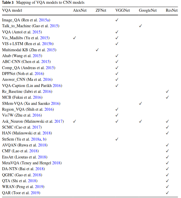
From the survey above, it's clear that VGGNet was the network of choice before ResNets came along. Most of the VQA papers that came out after 2017 use ResNets.

The core idea of ResNets involve skip connections, as shown below.

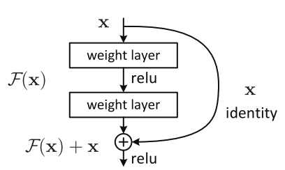
The identity shortcut connection allows the network to skip middle layers. The idea is to avoid exploding and vanishing gradients that very deep neural networks often face by allowing the network to skip layers if needed. It also helps improve accuracy, since layers hurting the accuracy can be skipped and regularized.

Ilievski et al. (2016) utilize question word embeddings (which we will discuss soon) to extract objects whose labels are similar to the question itself, and extract the feature representations of those objects using a ResNet. They call this approach "focused dynamic attention."

Lu et al. (2019) utilize ViLBERT (short for Vision-And-Language BERT) for visual question answering. ViLBERT consists of two parallel BERT-style models operating over image regions and text segments.  Each stream is a series of transformer and co-attentional transformer layers which enable information exchange between modalities.

Question Featurization

There are several methods to create embeddings. Older approaches include count-based, frequency-based methods like count vectorization and TF-IDF. There are prediction-based methods like continuous bag of words and skip grams as well. Pretrained models for the Word2Vec algorithm are also available in open source tools like Gensim. You can learn about these methods here. Deep learning architectures like RNNs, LSTMs, GRUs, and 1-D CNNs can also be used to create word embeddings. In VQA literature, LSTMs are used most frequently.

Most of you reading this article are probably already aware of what RNNs are, but we will still touch up on the basic concepts for the sake of completeness. Recurrent neural networks take in sequential inputs and predict the next element in the sequence depending on the data they’ve been trained on. Vanilla recurrent networks would, based on the input provided, process their previous hidden state and output the next hidden state and a sequential prediction. This prediction is compared with the ground truth values to update weights using backpropagation.

We also know that RNNs are susceptible to vanishing and exploding gradients. To fix this problem, LSTMs came into being. LSTMs use different gates to manage the amount of importance given to each previous element in the sequence. There are also bidirectional variants of LSTMs which learn the sequential dependence of different elements from left to right, as well as right to left.

Lu et al. (2016) build a hierarchical architecture that co-attends to the image and question at three levels: (a) the word level, (b) the phrase level, and (c) the question level. At the word level, they embed words to a vector space through an embedding matrix. At the phrase level, 1-dimensional convolutional neural networks are used to capture the information contained in unigrams, bigrams, and trigrams. At the question level, they use recurrent neural networks to encode the entire question.

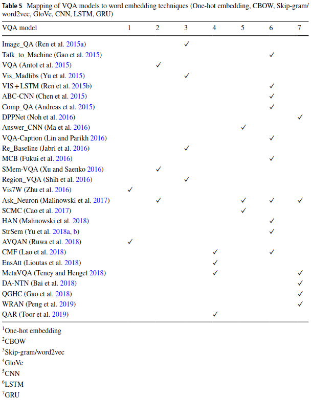
This survey lists unique ways of doing question featurization, which are also mentioned below.

Antol et al. (2015) use a BoW approach, but use only the top 1000 words from the questions in their dataset. They exploit the strong correlation between the words that start a question, and answer by creating another BoW from the top 10 first, second, and third words of the question, then concatenating it with the first representation.

Zhang et al. (2016) attempt to solve the binary visual question answering problem. They attempt to organize the information in a question by introducing a PRS structure, where P represents the primary object, R stands for relation, and S stands for the secondary object. P and S values would ideally be nouns, and the R would be verbs or prepositions.

To solve multiple-choice question answering, Shih et al. (2016) turned variable length questions into fixed-sized vectors by binning the words into the following categories:

• Type of question, using first two words
• Nominal subject
• All noun words
• All remaining words

Yu et al. (2018) leverage Tree-LSTMs to capture the semantics in the question and its relation with the image. Tree-LSTMs are tree-structured objects, where each node is an LSTM cell. The forward pass can be done in many ways:

• Child Sum Tree Unit: here the hidden states of the children nodes are added to get the output
• Child Max Pooling Unit: here the output is the maximum of all the child nodes
• Child Convolve + Max Pooling Unit: here the output is the maximum of the convolutions between different child nodes. A discrete convolution between two functions $f$ and $g$ can be represented as follows:

$$ (f * g)[n] = \sum_{m=-M}^{M} f[n - m]  g[m] $$

Each question in the dataset is parsed and mapped to a tree structure where the root node is set to the question sequence. The tree structure provides semantic structure that aids logical reasoning.

Toor et al. (2019) devised a method to understand the relevance of a question and also make edits to an irrelevant question that has proved effective. They call the method Question Action Relevance and Editing.

Joint Feature Representation

One of the most common ways of handling the different feature vectors coming from images and text is by just concatenating the two and letting later layers find the right weights for each. You can also try element-wise addition and multiplication, if the feature vectors are of the same length. Malinowski et al. (2017) tried all the methods mentioned above and found that element-wise multiplication gives the best accuracy. Shih et al. (2016) use a dot product, whereas Saito et al. (2017) use a hybrid approach. They concatenate the result from element-wise multiplication and element-wise addition.

Several papers have used Canonical Correlation Analysis to find joint feature representations as well. Canonical Correlation Analysis is a method of finding correlations between two independent sets of vectors. You can evaluate different linear combinations of both vectors, similar to what is done in PCA.

Let $X$ be a vector of length $p$. Then,

$$ U_{1} = a_{11}X_{1} + a_{12}X_{2} + ... + a_{1p}X_{p} $$

$$ U_{2} = a_{21}X_{1} + a_{22}X_{2} + ... + a_{2p}X_{p} $$

                                  ...                                     ...

$$ U_{p} = a_{p1}X_{1} + a_{p2}X_{2} + ... + a_{pp}X_{p} $$

Let $Y$ be a vector of length $q$. Then,

$$ V_{1} = b_{11}Y_{1} + b_{12}Y_{2} + ... + b_{1q}Y_{q} $$

$$ V_{2} = b_{21}Y_{1} + b_{22}Y_{2} + ... + b_{2q}Y_{q} $$

                                 ...                                     ...

$$ V_{q} = b_{q1}Y_{1} + b_{q2}Y_{2} + ... + b_{qq}Y_{q} $$

Then $ (U_{i}, V_{i}) $ is the $ i^{th} $ canonical variate pair. Out of the two vectors, you pick $X$ such that $p \leq q $ for computational convenience. Then there are $p$ canonical covariate pairs.

Covariance can be defined as follows:

$$ cov(x, y) = \frac{\sum (x_{i} - \bar{x})(y_{i} - \bar{y})}{N - 1}$$

We can compute the variances of $ U_{i} $ and $ V{i} $:

$$ var(U_{i}) = \sum_{k=1}^{p} \sum_{l=1}^{p} a_{ik}a_{il} cov(X_{k}, X_{l}) $$

$$ var(V_{i}) = \sum_{k=1}^{q} \sum_{l=1}^{q} b_{ik}b_{il} cov(Y_{k}, Y_{l}) $$

Then canonical correlation between $ U_{i} $ and $ V_{i} $ can be calculated using the following formula:

$$ \rho_{i}^{*} = \frac{cov(U_{i}, V_{i})}{\sqrt{var(U_{i}) var(V_{i})}} $$

To find the joint feature representation we need to maximize the correlation between U and V, or the value of $ \rho $. In the scikit-learn implementation, this is accomplished in the Partial Least Squares algorithm. Kernel CCA is another variant which utilizes a Lagrangian-based solution. Gong et al. (2014), Yu et al. (2015), and Tomassi et al. (2019) all use some variant of CCA in the joint feature representation.

Noh et al. (2015) designed Dynamic Parameter Prediction Networks (DPPNets) for this task. They add a fully-connected layer after a question is vectorized using a GRU to dynamically assign weights to each question, before fusing with image features. They found this was challenging when the feature vectors had a large number of parameters. To circumvent this, they utilized a hashing mechanism to create a joint feature representation. They apply a hashing trick proposed by Chen et al. (2015) for compression of neural networks. A hashing algorithm is used to group different parameters, and each group of parameters shares the same values. The hashing trick drastically reduces model sizes by exploiting redundancies in a neural network without hurting the model performance in any significant manner.

Fukui et al. (2016) utilize multi-modal bilinear pooling for joint feature creation. Bilinear models take the outer product of two vectors to generate a higher dimensional matrix, in which each parameter of a vector interacts with the parameters of another in a multiplicative manner. For large vector sizes, this can create huge models with too many trainable parameters.

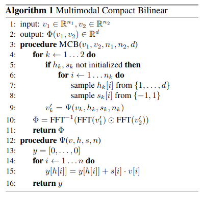
To avoid this, they use something called the Count Sketch Projection Function (as proposed by Charikar et al. (2002)), an algorithm designed to find the most frequent values in a data stream, and Fourier Transforms. In Count Sketch Projection, two vectors are initialized, one with -1 and 1 values and another that maps an input at index $i$ to an output at index $j$. For every element in the input, its destination index is looked up using the second vector we initialized earlier, and a dot product of the first vector with the input vector is added to the output. The Convolution Theorem states that a convolution between two vectors in the time domain is the same as an element-wise product in the frequency domain, which can be acquired by the Fourier Transform. They utilize this property of convolutions to finally get their joint representation. Hedi et al. (2017) also utilize multimodal compact bilinear pooling in their implementation of MUTAN for VQA.

Lu et al. (2016) use a co-attention mechanism before fusing the embeddings, so that visual attention and textual attention are both calculated. They suggest two attention mechanisms: parallel co-attention and alternating co-attention.

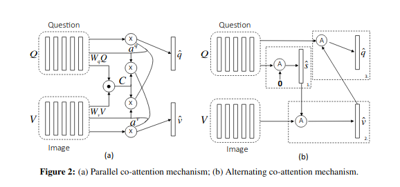
In parallel co-attention, they connect the image and question by calculating the similarity between image and question features at all pairs of image locations and question locations. They call the subsequent representation an affinity matrix. They use this affinity matrix to predict the attention maps.

$$ C = tanh(Q^{T}W_{b}V) $$

Here $C$ is the affinity matrix, $Q$ is the question feature vector, and $V$ is the vector of visual features. $W$ represents the weights.

$$ H_{v}= tanh(W_{v}V + (W_{q}Q)C) $$

$$ H_{q}= tanh(W_{q}Q + (W_{v}V)C^{T}) $$

$$ a_{v} = softmax(w^{T}_{hv} H^{v}) $$

$$ a_{q} = softmax(w^{T}_{hq} H^{q}) $$

Where $W_{v}$, $W_{q}$, $w_{hv}$, and $ w_{hq}$ are the weight parameters. $ a_{v} $ and $ a_{q} $ are the attention probabilities for each image region $ v_{n} $ and word $ q_{t} $, respectively.

$$ v = \sum_{n=1}^{N} a^{v}_{n} v_{n} ,  q = \sum_{t=1}^{T} a^{q}_{t} q_{t} $$

Where $v$ and $q$ are the parallel co-attention vectors for the image and the question, respectively.

They also propose alternating co-attention, where they sequentially alternate between generating image and question attention. The image features influence the question attention and vice-versa.

$$ H = tanh(W_{x}X+ (W_{g}g)1^{T}) $$

$$ a_{x} = softmax(w^{T}_{hx} H) $$

$$ x=\sum a^{x}_{i} x_{i} $$

Where $1$ is a vector with all elements being $1$. $ W_{x} $, $ W_{g} $, and $ w_{hx} $ are parameters. $ a_{x} $ is the attention weight of feature $X$.

In a very clever fashion, Kim et al. (2016) use residual connections for joint feature representations extracted from a CNN-based architecture for image featurization, and an LSTM architecture for question featurization. The Multimodal Residual Network architecture looks something like this.

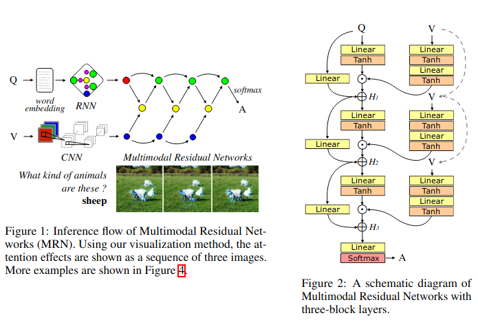
The residual connections add an attention ability to the network that the authors have visualized as well.

Gao et al. (2018) realized that a lot of spatial information is lost when we take only the one-dimensional vector representation from the 2nd to last layer of some convolutional networks, like ResNet. To solve for this, they use what they call "question guided hybrid convolutions", where they create convolutional kernels that take question representations created using a GRU along with the ResNet feature vectors to create a joint feature representation.

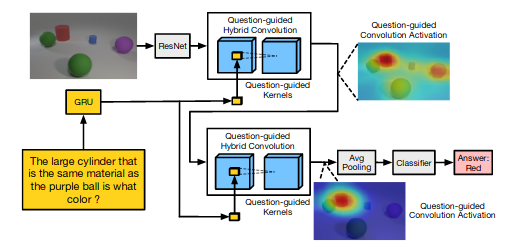
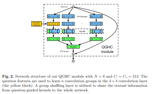
The authors point out that to predict a commonly used $(3×3×256×256)$ kernel from a 2000-D question feature vector, the fully-connected layer for learning the mapping generates 117 million parameters, which is hard to learn and causes overfitting on existing VQA datasets. To tackle that, they try to predict group convolutional kernel parameters instead. The QGHC module looks something like this.

Peng et al. (2019) proposed that the entire feature vector generated by an LSTM is not needed. Only keywords need to be extracted from the question. They utilize this idea and proposed a Word-to-Region Attention Network (WRAN), which can locate relevant object regions and identify the corresponding words in the reference question.

Answer Generation

The research on VQA includes (source):

• Free-form, open-ended questions where the answer could be words, phrases, and even complete sentences
• Object counting questions, where the answer involves counting the number of objects in one image
• Multi-choice questions
• Binary questions (yes/no)

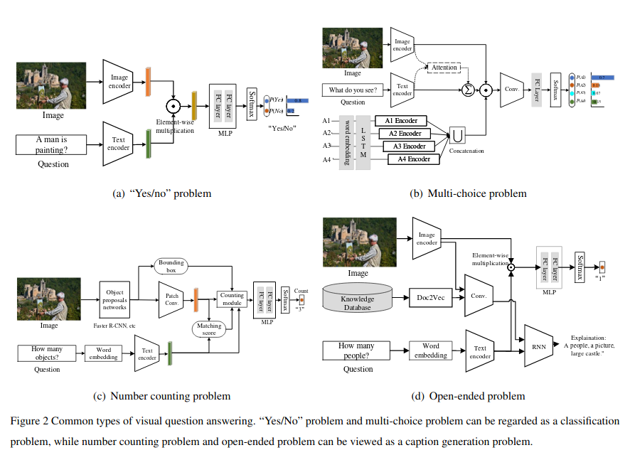
Binary questions and multiple choice questions often utilize a sigmoid layer at the end. The joint representations are passed through one or two fully-connected layers. The output is passed through a single neuron layer which functions as the classification layer.

For multiple choice questions, the answer choices are encoded using some embedding generation mechanism like the ones we discussed earlier. This is fed into the mechanism of joint feature generation. The joint feature is then passed through a fully-connected layer, and finally a multiclass classification layer with a softmax activation function.

For free-form, open-ended questions, the joint feature representations are converted into answers usually using a recurrent network like LSTMs. Wu et al. (2016) extract data about the image to provide the language model with more context. They use the Doc2Vec algorithm to get embeddings, which are used along with an LSTM to generate answers. Malinowski et al. (2017) devise a method in which the image feature is fed along with each word's representation as encoded by an LSTM.

Ruwa et al. (2018) use not just image and question features, but also take mood embeddings into account. A CNN-based mood detector is trained concurrently with the LSTM attention model in relation to local regions of an image. The mood relates to the appearance and actions of people in the images.

Datasets

There are a lot of datasets that address different kinds of tasks in the visual question answering domain. Some of the primary ones are discussed here.

• DAQUAR (Dataset for Question Answering on Real World Images) is a dataset of human question-answer pairs about images.
• COCO-QA is an extension of the COCO (Common Objects in Context) dataset. The questions are of 4 different types: object, number, color, and location. All answers are of a single-word type.
• VQA dataset, which is larger than other datasets. In addition to the 204,721 images from the COCO dataset, it includes 50,000 abstract cartoon images. There are three questions per image and ten answers per question. The dataset includes multiple choice answers, as well open-ended answers.
• Visual Madlibs has over 10,000 images which have 12 fill-in-the-blanks types in the dataset. It provides two evaluation methods: multiple choice questions and fill in the blanks.
• Visual7W dataset contains seven types of questions: what, where, when, who, why, how, and which. The dataset was collected on 47,300 COCO images. In total, it has 327,939 QA pairs, together with 1,311,756 human-generated multiple-choices, and 561,459 object groundings from 36,579 categories. In addition, they provide complete grounding annotations that link the object mentions in the QA sentences to their bounding boxes in the images, and therefore introduce a new QA type with image regions as the visually grounded answers. They also provide a toolkit for developers and AI researchers.
• CLEVR dataset consists of a training set of 70,000 images and 699,989 questions, a validation set of 15,000 images and 149,991 questions, a test set of 15,000 images and 14,988 questions, as well as answers for all train and validation questions. Besides that, they also provide scene graph annotations for train and val images giving ground truth locations, attributes, and relationships for objects.
• Visual Genome has 1.7 million visual question answers in their dataset. Besides VQA, they provide a lot of other kind of data as well–region descriptions, object instances, and all the annotations mapped to WordNet synsets.

Evaluation Metrics

In multiple choice tasks, simple accuracy is enough to evaluate a given VQA model. But for open-ended VQA tasks, the framework of an exact string match would be a very rigid way to evaluate the performance of the VQA model.

Wu and Palmer Similarity

Wu and Palmer Similarity utilizes fuzzy logic to calculate the similarity between two phrases. This is a score that takes into account the position of concepts $ c_{1} $ and $ c_{2} $ in the taxonomy, relative to the position of the Least Common Subsumer ($ c_{1} $, $ c_{2} $). It assumes that the similarity between two concepts is the function of path length and depth in path-based measures.

The Least Common Subsumer of two nodes $v$ and $w$ in a tree or directed acyclic graph (DAG) is the deepest node that has both $v$ and $w$ as descendants, where we define each node to be a descendant of itself. So if $v$ has a direct connection from $w$, $w$ is the lowest common ancestor.

$$ Sim_{wup}(c_{1}, c_{2}) = 2*  \frac{Depth(LCS(c_{1}, c_{2}))}{(Depth(c_{1}) + Depth(c_{2}))} $$

$ LCS(c_{1}, c_{2}) $ = lowest node in the hierarchy that is a hypernym of $ c_{1} $, $ c_{2} $.

NLTK has a function that implements WUP similarity.

WUP similarity works for single-word answers, but doesn't work for phrases or sentences.

BLEU (Bilingual Evaluation Understudy)

This approach works by counting matching n-grams in the candidate translation to n-grams in the reference text. The comparison is made regardless of word order.

$$ P_{n} = \frac{\sum_{n-grams} count_{clip}(n-gram)}{\sum_{n-grams} count(n-gram)} $$

They also have a brevity penalty attached to the score, which is defined as follows.

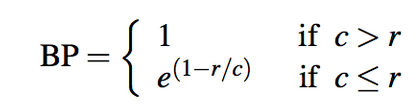
Where $r$ is the length of the reference answer and $c$ is the length of the prediction.

$$ BLEU = BP * exp( \sum_{n=1}^{N}W_{n}logP_{n}) $$

A comprehensive guide to the BLEU metric can be found in this this article.

BLEU has some drawbacks, too. To a great extent, the BLEU score is based on very simplistic text string matches. Very roughly, the larger the cluster of words that you can match exactly, the higher the BLEU score. This makes it not the best metric if the answers are long and can go beyond small phrases. The NLTK implementation tutorial can be found here.

METEOR (Metric for evaluation of translation with explicit ordering)

The METEOR metric has two parts to its calculations. First, it calculates the precision and recall for all unigrams. Then it takes a harmonic mean of the precision and $9 \times$ the recall.

$$ F_{mean} = \frac{10PR}{P + 9R} $$

Precision and recall are calculated based on unigram matches.

To take into account longer matches, METEOR computes a penalty for a given alignment as follows. First, all the unigrams in the system translation that are mapped to unigrams in the reference translation are grouped into the fewest possible number of chunks, such that the unigrams in each chunk are in adjacent positions in the system translation, and are also mapped to unigrams that are in adjacent positions in the reference translation.

The second part is a penalty function that is formulated as follows:

$$ penalty = 0.5 * (\frac{\text{number of chunks}}{\text{number of unigrams}})^{3} $$

Finally, the score is:

$$ score = F_{mean} * (1 - penalty) $$

Conclusion

Here we've covered a survey of the progress in the field of visual question answering. We understood that the problem is divided into four main areas of research: image featurization, question featurization, joint feature representation, and answer generation. After reviewing each, we saw an overview of several different approaches that many researchers have used to tackle these problems in recent years. We also took a look at the major datasets and evaluation metrics for the task of visual question answering. I hope you found the article useful.