In this tutorial we extend our implementation of gradient descent to work with a single hidden layer with any number of neurons.

Part 4 is divided into two sections. In the first we will extend the implementation of Part 3 to allow for 5 neurons in a single hidden layer, rather than just 2. The second section will address making the gradient descent (GD) algorithm neuron-agnostic, in that any number of hidden neurons can be included within a single hidden layer.

This is the fourth part in a tutorial series dedicated to showing you how to implement a generic gradient descent algorithm in Python. This can be implemented for any neural network architecture to optimize its parameters. In Part 2 we saw how to implement the GD algorithm for any number of input neurons. In Part 3 we extended this implementation to work for an additional single layer with 2 neurons. At the end of this part of the tutorial there will be an implementation of the gradient descent algorithm in Python which works with any number of inputs, and a single hidden layer with any number of neurons.

Step 1: 1 Hidden Layer with 5 Neurons

We will begin by extending the previous implementation to allow for 5 neurons in the hidden layer. This is show schematically below in the figure below. A simple way to extend the algorithm is just by repeating some lines of code we already wrote, now for all 5 neurons.

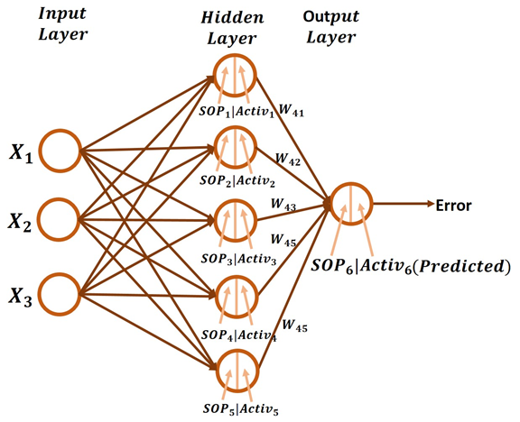
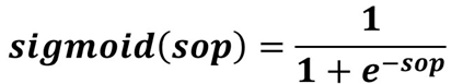
Before taking a look at the backward pass, it is worth recalling that in the forward pass the sigmoid activation function is used (defined below). Note that SOP stands for sum of products.

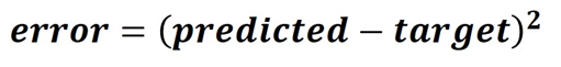
The error is calculated using the standard squared error function.

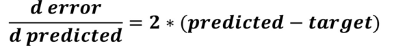
In the backward pass, the gradients for updating the weights between the hidden layer and the output layer are simply calculated as discussed in Part 3, without any change. The first derivative is the error to predicted output derivative given below.

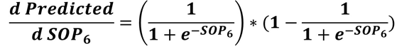
The second derivative is the predicted output to SOP6 derivative.

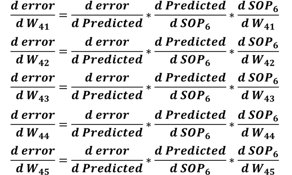
The third and last derivative is the SOP6 to the weights between the hidden and output layers. Because there are 5 weights connecting the 5 hidden neurons to the output neuron, then there will be 5 derivatives, one for each weight. Remember that SOP6 is calculated according to the equation below:

SOP6 = Activ1*W41 + Activ2*W42 + Activ3*W43 + Activ4*W44 + Activ5*W45

For example, the derivative of SOP6 to W41 is equal to Activ1, the SOP6 to W42 derivative is equal to Activ2, and so on.

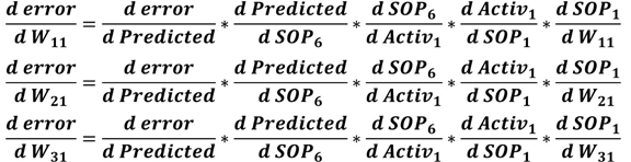
In order to calculate the gradients for such 5 weights, the chain of the previous 3 derivatives will be multiplied. All gradients are calculated according to the equations in the next figure. All of these gradients share the first 2 derivatives in the chain.

After calculating the gradients for the weights between the hidden and output layers, next is to calculate the gradients for the weights between the input and hidden layers.

The derivative chain for calculating such gradients will start by the first 2 derivatives previously calculated which are:

1. Error to predicted output derivative.
2. Predicted output to SOP6 derivative.

The third derivative in the chain will be the SOP6 to the output of the sigmoid function (Activ1 to Activ5). Based on the equation that relates both SOP6 and Activ1 to Activ2, which is given below again, the SOP6 to Activ1 derivative is equal to W41, the SOP6 to Activ2 derivative is W42, and so on.

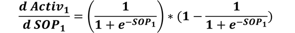
SOP6 = Activ1*W41 + Activ2*W42 + Activ3*W43 + Activ4*W44 + Activ5*W45

The next derivative in the chain is the derivative of the sigmoid function to the SOP in the hidden layer. For example, the Activ1 to SOP1 derivative is calculated according to the equation below. For calculating the derivative of Activ2 to SOP2, just replace SOP1 by SOP2. This applies to all other derivatives.

The last derivative in the chain is to calculate the derivative of the SOP at each hidden neuron with respect to the weights connected to it. For simplicity, the next figure shows the ANN architecture with all connections between the input layer and the hidden layer removed except for the connections to the first hidden neuron.

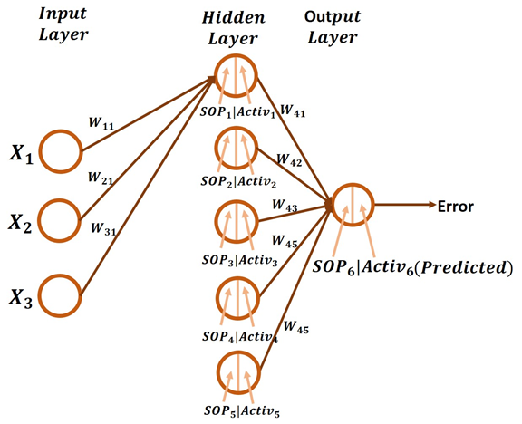
In order to calculate the derivative of SOP1 to its 3 weights which are W11, W21, and W31, we have to keep in mind the equation that relates all of them which is given below. As a result, the SOP1 to W11 derivative is X1, the SOP2 to W21 derivative is X2, and so on.

SOP1 = X1*W11 + X2*W21 + X3*W31

If the weights connecting the input neurons to the second hidden neuron are W12, W22, and W32, then SOP2 is calculated as given below. As a result, the SOP2 to W12 derivative is X1, SOP2 to W22 derivative is X2, and so on. The process continues for all other hidden neurons.

SOP2 = X1*W12 + X2*W22 + X3*W32

You might note that the result of the derivatives of any SOP to its 3 weights will be X1, X2, and X3.

After calculating all derivatives in the chain from the error to the input layer weights, we can calculate the gradients. For example, the 3 gradients of the 3 weights connected to the first hidden neuron are calculated according to the equations listed below. Note that all chains share the same derivatives except for the final derivative.

For working with the second hidden neuron, each Activ1 is replaced by Activ2 and each SOP1 is replaced by SOP2. This is also valid for working with other hidden neurons.

At this point, we successfully prepare all derivative chains for calculating the gradients for all weights in the network. Next is to implement that in Python.

Python Implementation

The Python script for implementing the GD algorithm for optimizing an ANN with 3 inputs and a hidden layer with 5 neurons is listed below. We will discuss each part of this code.

import numpy

def sigmoid(sop):
    return 1.0 / (1 + numpy.exp(-1 * sop))

def error(predicted, target):
    return numpy.power(predicted - target, 2)

def error_predicted_deriv(predicted, target):
    return 2 * (predicted - target)

def sigmoid_sop_deriv(sop):
    return sigmoid(sop) * (1.0 - sigmoid(sop))

def sop_w_deriv(x):
    return x

def update_w(w, grad, learning_rate):
    return w - learning_rate * grad

x = numpy.array([0.1, 0.4, 4.1])
target = numpy.array([0.2])

learning_rate = 0.001

w1_3 = numpy.random.rand(3)
w2_3 = numpy.random.rand(3)
w3_3 = numpy.random.rand(3)
w4_3 = numpy.random.rand(3)
w5_3 = numpy.random.rand(3)
w6_5 = numpy.random.rand(5)
w6_5_old = w6_5
print("Initial W : ", w1_3, w2_3, w3_3, w4_3, w5_3, w6_5)

# Forward Pass
# Hidden Layer Calculations
sop1 = numpy.sum(w1_3 * x)
sop2 = numpy.sum(w2_3 * x)
sop3 = numpy.sum(w3_3 * x)
sop4 = numpy.sum(w4_3 * x)
sop5 = numpy.sum(w5_3 * x)

sig1 = sigmoid(sop1)
sig2 = sigmoid(sop2)
sig3 = sigmoid(sop3)
sig4 = sigmoid(sop4)
sig5 = sigmoid(sop5)

# Output Layer Calculations
sop_output = numpy.sum(w6_5 * numpy.array([sig1, sig2, sig3, sig4, sig5]))

predicted = sigmoid(sop_output)
err = error(predicted, target)

# Backward Pass
g1 = error_predicted_deriv(predicted, target)

### Working with weights between hidden and output layer
g2 = sigmoid_sop_deriv(sop_output)

g3 = numpy.zeros(w6_5.shape[0])
g3[0] = sop_w_deriv(sig1)
g3[1] = sop_w_deriv(sig2)
g3[2] = sop_w_deriv(sig3)
g3[3] = sop_w_deriv(sig4)
g3[4] = sop_w_deriv(sig5)

grad_hidden_output = g3 * g2 * g1

w6_5[0] = update_w(w6_5[0], grad_hidden_output[0], learning_rate)
w6_5[1] = update_w(w6_5[1], grad_hidden_output[1], learning_rate)
w6_5[2] = update_w(w6_5[2], grad_hidden_output[2], learning_rate)
w6_5[3] = update_w(w6_5[3], grad_hidden_output[3], learning_rate)
w6_5[4] = update_w(w6_5[4], grad_hidden_output[4], learning_rate)

### Working with weights between input and hidden layer
# First Hidden Neuron
g3 = sop_w_deriv(w6_5_old[0])
g4 = sigmoid_sop_deriv(sop1)
g5 = sop_w_deriv(x)
grad_hidden1_input = g5 * g4 * g3 * g2 * g1
w1_3 = update_w(w1_3, grad_hidden1_input, learning_rate)

# Second Hidden Neuron
g3 = sop_w_deriv(w6_5_old[1])
g4 = sigmoid_sop_deriv(sop2)
g5 = sop_w_deriv(x)
grad_hidden2_input = g5 * g4 * g3 * g2 * g1
w2_3 = update_w(w2_3, grad_hidden2_input, learning_rate)

# Third Hidden Neuron
g3 = sop_w_deriv(w6_5_old[2])
g4 = sigmoid_sop_deriv(sop3)
g5 = sop_w_deriv(x)
grad_hidden3_input = g5 * g4 * g3 * g2 * g1
w3_3 = update_w(w3_3, grad_hidden3_input, learning_rate)

# Fourth Hidden Neuron
g3 = sop_w_deriv(w6_5_old[3])
g4 = sigmoid_sop_deriv(sop4)
g5 = sop_w_deriv(x)
grad_hidden4_input = g5 * g4 * g3 * g2 * g1
w4_3 = update_w(w4_3, grad_hidden4_input, learning_rate)

# Fourth Hidden Neuron
g3 = sop_w_deriv(w6_5_old[4])
g4 = sigmoid_sop_deriv(sop5)
g5 = sop_w_deriv(x)
grad_hidden5_input = g5 * g4 * g3 * g2 * g1
w5_3 = update_w(w5_3, grad_hidden5_input, learning_rate)

w6_5_old = w6_5
print(predicted)

Preparing the inputs and their output is the first thing done in this code according to the lines below. Because the input layer has 3 inputs, then just an array with 3 values exist. It is not actually an array but a vector. The target is specified as a single value.

x = numpy.array([0.1, 0.4, 4.1])
target = numpy.array([0.2])

Next is to prepare the network weights as given below. The weights of each hidden neuron are created in a separate variable. For example, the weights of the first hidden neuron are stored into the w1_3 variable. The variable w6_5 holds the 5 weights connecting the 5 hidden neurons to the output neuron.

w1_3 = numpy.random.rand(3)
w2_3 = numpy.random.rand(3)
w3_3 = numpy.random.rand(3)
w4_3 = numpy.random.rand(3)
w5_3 = numpy.random.rand(3)
w6_5 = numpy.random.rand(5)

The variable w6_5_old holds the weights in the w6_5 variable as a backup for use when calculating the SOP6 to Activ1-Activ5 derivatives.

w6_5_old = w6_5

After preparing the inputs, outputs, and weights, next is to start the forward pass. The first task is to calculate the SOP for each hidden neuron as given below. This is by multiplying the 3 inputs by the 3 weights.

# Forward Pass
# Hidden Layer Calculations
sop1 = numpy.sum(w1_3 * x)
sop2 = numpy.sum(w2_3 * x)
sop3 = numpy.sum(w3_3 * x)
sop4 = numpy.sum(w4_3 * x)
sop5 = numpy.sum(w5_3 * x)

After that, the sigmoid function is applied to all of these sums of products.

sig1 = sigmoid(sop1)
sig2 = sigmoid(sop2)
sig3 = sigmoid(sop3)
sig4 = sigmoid(sop4)
sig5 = sigmoid(sop5)

The outputs of the sigmoid function are regarded the inputs to the output neuron. The SOP for such a neuron is calculated using the line below.

# Output Layer Calculations
sop_output = numpy.sum(w6_5 * numpy.array([sig1, sig2, sig3, sig4, sig5]))

The SOP of the output neuron is fed to the sigmoid function to return the predicted output. After the predicted output is calculated, next is to calculate the error using the error() function. Error calculation is the final step in the forward pass. Next is to start the backward pass.

predicted = sigmoid(sop_output)
err = error(predicted, target)

In the backward pass, the first derivative calculated is the error to the predicted output derivative according to the line below. The result is saved in the variable g1 for later use.

g1 = error_predicted_deriv(predicted, target)

The next derivative is the predicted output to SOP6 derivative according to the next line. The result is saved in the variable g2 for later use.

g2 = sigmoid_sop_deriv(sop_output)

In order to calculate the gradients of the weights between the hidden and output layers, the remaining derivative is the SOP6 to W41-W45 derivatives. They are calculated in the variable g3 according to the next lines.

g3 = numpy.zeros(w6_5.shape[0])
g3[0] = sop_w_deriv(sig1)
g3[1] = sop_w_deriv(sig2)
g3[2] = sop_w_deriv(sig3)
g3[3] = sop_w_deriv(sig4)
g3[4] = sop_w_deriv(sig5)

After preparing all derivatives required for calculating the gradients for the weights W41 to W45, next is to calculate the gradients using the next line.

grad_hidden_output = g3 * g2 * g1

After that, such 5 weights can be updated using the update_w() function as given below. It accepts the old weights, gradients, and learning rate and returns the new weights.

w6_5 = update_w(w6_5, grad_hidden_output, learning_rate)

After updating the weights between the hidden and output layers, next is to calculate the gradients for the weights between the input and hidden layers. Through our discussion, we will work on a single hidden neuron at a time.

For the first hidden neuron, the required calculations for preparing the gradients for its weights are given below. In the variable g3, the SOP6 to Activ1 derivative is calculated. In g4, the Activ1 to SOP1 derivative is calculated. The last derivatives are the SOP1 to W11-W31 derivatives which are saved in the g5 variable. Note that g5 has 3 derivatives, one for each weight while g4 and g3 has just one derivative.

After calculating all derivatives in the chain, next is to calculate the gradient for updating the 3 weights connecting the 3 input neurons to the first hidden neuron by multiplying the variables g1 to g5. The result is saved in the grad_hidden1_input variable. Finally, the 3 weights are updated using the update_w() function.

# First Hidden Neuron
g3 = sop_w_deriv(w6_5_old[0])
g4 = sigmoid_sop_deriv(sop1)
g5 = sop_w_deriv(x)
grad_hidden1_input = g5 * g4 * g3 * g2 * g1
w1_3 = update_w(w1_3, grad_hidden1_input, learning_rate)

Working on the other hidden neurons is very similar to the above code. From the above 5 lines, just changes are necessary for the first 2 lines. For working with the second hidden neuron, use index 1 for w6_5_old for calculating g3. For calculating g4, use sop2 rather than sop1. The part of the code responsible for updating the weights of the second hidden neuron is listed below.

# Second Hidden Neuron
g3 = sop_w_deriv(w6_5_old[1])
g4 = sigmoid_sop_deriv(sop2)
g5 = sop_w_deriv(x)
grad_hidden2_input = g5 * g4 * g3 * g2 * g1
w2_3 = update_w(w2_3, grad_hidden2_input, learning_rate)

For working with the third hidden neuron, use index 2 for w6_5_old for calculating g3. For calculating g4, use sop3. Its code is given below.

# Third Hidden Neuron
g3 = sop_w_deriv(w6_5_old[2])
g4 = sigmoid_sop_deriv(sop3)
g5 = sop_w_deriv(x)
grad_hidden3_input = g5 * g4 * g3 * g2 * g1
w3_3 = update_w(w3_3, grad_hidden3_input, learning_rate)

For working with the forth hidden neuron, use index 3 for w6_5_old for calculating g3. For calculating g4, use sop4. Its code is given below.

# Fourth Hidden Neuron
g3 = sop_w_deriv(w6_5_old[3])
g4 = sigmoid_sop_deriv(sop4)
g5 = sop_w_deriv(x)
grad_hidden4_input = g5 * g4 * g3 * g2 * g1
w4_3 = update_w(w4_3, grad_hidden4_input, learning_rate)

For working with the fifth and final hidden neuron, use index 4 for w6_5_old for calculating g3. For calculating g4, use sop5. Its code is given below.

# Fifth Hidden Neuron
g3 = sop_w_deriv(w6_5_old[4])
g4 = sigmoid_sop_deriv(sop5)
g5 = sop_w_deriv(x)
grad_hidden5_input = g5 * g4 * g3 * g2 * g1
w5_3 = update_w(w5_3, grad_hidden5_input, learning_rate)

At this point, the gradients for all network weights are calculated and the weights are updated. Just remember to set the w6_5_old variable to the new w6_5 at the end.

w6_5_old = w6_5

After implementing the GD algorithm for the architecture in use, we can allow the algorithm to be applied in a number of iterations using a loop. This is implemented in the code listed below.

import numpy

def sigmoid(sop):
    return 1.0/(1+numpy.exp(-1*sop))

def error(predicted, target):
    return numpy.power(predicted-target, 2)

def error_predicted_deriv(predicted, target):
    return 2*(predicted-target)

def sigmoid_sop_deriv(sop):
    return sigmoid(sop)*(1.0-sigmoid(sop))

def sop_w_deriv(x):
    return x

def update_w(w, grad, learning_rate):
    return w - learning_rate*grad

x = numpy.array([0.1, 0.4, 4.1])
target = numpy.array([0.2])

learning_rate = 0.001

w1_3 = numpy.random.rand(3)
w2_3 = numpy.random.rand(3)
w3_3 = numpy.random.rand(3)
w4_3 = numpy.random.rand(3)
w5_3 = numpy.random.rand(3)
w6_5 = numpy.random.rand(5)
w6_5_old = w6_5
print("Initial W : ", w1_3, w2_3, w3_3, w4_3, w5_3, w6_5)

for k in range(80000):
    # Forward Pass
    # Hidden Layer Calculations
    sop1 = numpy.sum(w1_3*x)
    sop2 = numpy.sum(w2_3*x)
    sop3 = numpy.sum(w3_3*x)
    sop4 = numpy.sum(w4_3*x)
    sop5 = numpy.sum(w5_3*x)
    
    sig1 = sigmoid(sop1)
    sig2 = sigmoid(sop2)
    sig3 = sigmoid(sop3)
    sig4 = sigmoid(sop4)
    sig5 = sigmoid(sop5)

    # Output Layer Calculations
    sop_output = numpy.sum(w6_5*numpy.array([sig1, sig2, sig3, sig4, sig5]))

    predicted = sigmoid(sop_output)
    err = error(predicted, target)
    
    # Backward Pass
    g1 = error_predicted_deriv(predicted, target)

    ### Working with weights between hidden and output layer
    g2 = sigmoid_sop_deriv(sop_output)
    
    g3 = numpy.zeros(w6_5.shape[0])
    g3[0] = sop_w_deriv(sig1)
    g3[1] = sop_w_deriv(sig2)
    g3[2] = sop_w_deriv(sig3)
    g3[3] = sop_w_deriv(sig4)
    g3[4] = sop_w_deriv(sig5)
    
    grad_hidden_output = g3*g2*g1
    
    w6_5 = update_w(w6_5, grad_hidden_output, learning_rate)

    ### Working with weights between input and hidden layer
    # First Hidden Neuron
    g3 = sop_w_deriv(w6_5_old[0])
    g4 = sigmoid_sop_deriv(sop1)
    g5 = sop_w_deriv(x)
    grad_hidden1_input = g5*g4*g3*g2*g1
    w1_3 = update_w(w1_3, grad_hidden1_input, learning_rate)

    # Second Hidden Neuron
    g3 = sop_w_deriv(w6_5_old[1])
    g4 = sigmoid_sop_deriv(sop2)
    g5 = sop_w_deriv(x)
    grad_hidden2_input = g5*g4*g3*g2*g1
    w2_3 = update_w(w2_3, grad_hidden2_input, learning_rate)
    
    # Third Hidden Neuron
    g3 = sop_w_deriv(w6_5_old[2])
    g4 = sigmoid_sop_deriv(sop3)
    g5 = sop_w_deriv(x)
    grad_hidden3_input = g5*g4*g3*g2*g1
    w3_3 = update_w(w3_3, grad_hidden3_input, learning_rate)
    
    # Fourth Hidden Neuron
    g3 = sop_w_deriv(w6_5_old[3])
    g4 = sigmoid_sop_deriv(sop4)
    g5 = sop_w_deriv(x)
    grad_hidden4_input = g5*g4*g3*g2*g1
    w4_3 = update_w(w4_3, grad_hidden4_input, learning_rate)
    
    # Fifth Hidden Neuron
    g3 = sop_w_deriv(w6_5_old[4])
    g4 = sigmoid_sop_deriv(sop5)
    g5 = sop_w_deriv(x)
    grad_hidden5_input = g5*g4*g3*g2*g1
    w5_3 = update_w(w5_3, grad_hidden5_input, learning_rate)
    
    w6_5_old = w6_5
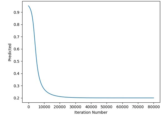
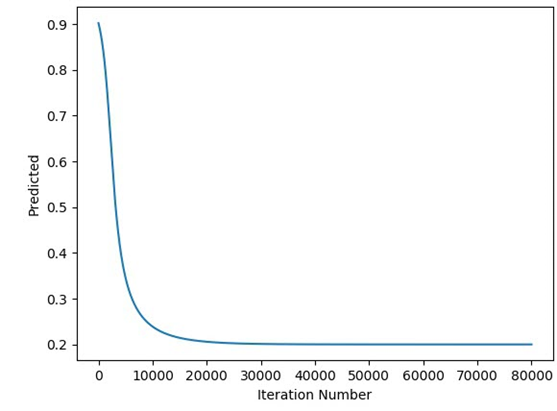
    print(predicted)

The figure below shows a plot relating the predicted output to each iteration.

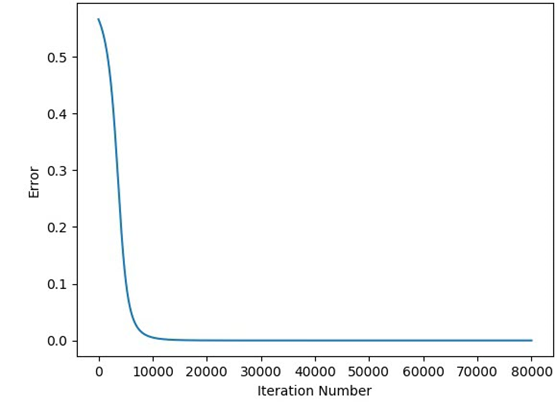
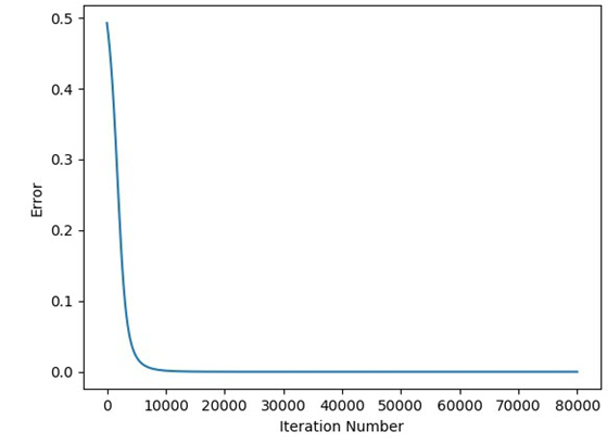
The relation between the error and the iteration is given in the next figure.

The previous GD algorithm implementation not only works for a single hidden layer but also for a specific number of neurons within that layer. Seeking to generalize the algorithm, we can continue editing the previous implementation so that it can work for any number of neurons within a single hidden layer. Later, more hidden layer could be added and the algorithm will not depend on a fixed number of hidden layers.

Step 2: Working with Any Number of Hidden Neurons

According to the previous implementation, the calculations for each neuron are nearly identical. The same code is used but just feeding it with the appropriate inputs. Using a loop, we can write such code once and use different inputs for each iteration. The new code is given below.

import numpy

def sigmoid(sop):
    return 1.0/(1+numpy.exp(-1*sop))

def error(predicted, target):
    return numpy.power(predicted-target, 2)

def error_predicted_deriv(predicted, target):
    return 2*(predicted-target)

def sigmoid_sop_deriv(sop):
    return sigmoid(sop)*(1.0-sigmoid(sop))

def sop_w_deriv(x):
    return x

def update_w(w, grad, learning_rate):
    return w - learning_rate*grad

x = numpy.array([0.1, 0.4, 4.1])
target = numpy.array([0.2])

learning_rate = 0.001

# Number of inputs, number of neurons per each hidden layer, number of output neurons
network_architecture = numpy.array([x.shape[0], 5, 1])

# Initializing the weights of the entire network
w = []
w_temp = []
for layer_counter in numpy.arange(network_architecture.shape[0]-1):
    for neuron_nounter in numpy.arange(network_architecture[layer_counter+1]):
        w_temp.append(numpy.random.rand(network_architecture[layer_counter]))
    w.append(numpy.array(w_temp))
    w_temp = []
w = numpy.array(w)
w_old = w
print("Initial W : ", w)

for k in range(10000000000000):
    # Forward Pass
    # Hidden Layer Calculations
    sop_hidden = numpy.matmul(w[0], x)

    sig_hidden = sigmoid(sop_hidden)

    # Output Layer Calculations
    sop_output = numpy.sum(w[1][0]*sig_hidden)

    predicted = sigmoid(sop_output)
    err = error(predicted, target)

    # Backward Pass
    g1 = error_predicted_deriv(predicted, target)

    ### Working with weights between hidden and output layer
    g2 = sigmoid_sop_deriv(sop_output)
    g3 = sop_w_deriv(sig_hidden)
    grad_hidden_output = g3*g2*g1
    w[1][0] = update_w(w[1][0], grad_hidden_output, learning_rate)
    
    ### Working with weights between input and hidden layer
    g5 = sop_w_deriv(x)
    for neuron_idx in numpy.arange(w[0].shape[0]):
        g3 = sop_w_deriv(w_old[1][0][neuron_idx])
        g4 = sigmoid_sop_deriv(sop_hidden[neuron_idx])
        grad_hidden_input = g5*g4*g3*g2*g1
        w[0][neuron_idx] = update_w(w[0][neuron_idx], grad_hidden_input, learning_rate)

    w_old = w
    print(predicted)

The inputs and the target are specified as previously done. There is a variable named network_architecture which holds the ANN architecture. For the architecture in use, the number of inputs equal to x.shape[0] which is 3 in this example, number of hidden neurons is 5, and number of output neurons is 1.

network_architecture = numpy.array([x.shape[0], 5, 1])

Using a for loop that goes through each layer specified in the architecture, the weights of the network can be created within a single array named w. The code is listed below. This is a better way of building the network weights compared to using individual variables for holding the weights of each individual layer.

# Initializing the weights of the entire network
w = []
w_temp = []
for layer_counter in numpy.arange(network_architecture.shape[0]-1):
    for neuron_nounter in numpy.arange(network_architecture[layer_counter+1]):
        w_temp.append(numpy.random.rand(network_architecture[layer_counter]))
    w.append(numpy.array(w_temp))
    w_temp = []
w = numpy.array(w)

For this example, the shape of the array w is (2,) which means there are just 2 elements within it. The shape of the first element is (5, 3) which holds the weights between the input layer, which has 3 inputs, and a hidden layer, which has 5 neurons. The shape of the second element in the array w is (1, 5) which holds the weights between the hidden layer which has 5 neurons and the output layer which has just a single neuron.

Preparing the weights this way facilitates working on both the forward and backward pass. All sum of products are calculated using a single line as follows. Note that w[0] means the weights between the input and hidden layers.

sop_hidden = numpy.matmul(w[0], x)

Similarly, the sigmoid function is called once to be applied to all sum of products as follows.

sig_hidden = sigmoid(sop_hidden)

The sum of products between the hidden and output layers are calculated according to this single line. Note that w[1] returns the weights between such 2 layers.

sop_output = numpy.sum(w[1][0]*sig_hidden)

As regular, the predicted output and the error are calculated as follows.

predicted = sigmoid(sop_output)
err = error(predicted, target)

This is the end of the forward pass. In the backward pass, because there is just a single neuron in the output layer, then its weights will be updated in the same way used previously.

# Backward Pass
g1 = error_predicted_deriv(predicted, target)

### Working with weights between hidden and output layer
g2 = sigmoid_sop_deriv(sop_output)
g3 = sop_w_deriv(sig_hidden)
grad_hidden_output = g3*g2*g1
w[1][0] = update_w(w[1][0], grad_hidden_output, learning_rate)

When working on updating the weights between the input and hidden layers, a for loop is used as given below. It loops through each neuron in the hidden layer and uses the appropriate inputs to the functions sop_w_deriv()and sigmoid_sop_deriv().

### Working with weights between input and hidden layer
g5 = sop_w_deriv(x)
for neuron_idx in numpy.arange(w[0].shape[0]):
    g3 = sop_w_deriv(w_old[1][0][neuron_idx])
    g4 = sigmoid_sop_deriv(sop_hidden[neuron_idx])
    grad_hidden_input = g5*g4*g3*g2*g1
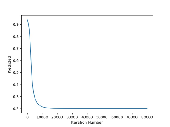
    w[0][neuron_idx] = update_w(w[0][neuron_idx], grad_hidden_input, learning_rate)

By doing so, we have successfully minimized the GD algorithm code and also generalized it to work with any number of hidden neurons within a single hidden layer. Before testing the code with different numbers of hidden neurons, let's make sure it works correctly as the previous implementation. The next figure shows how the predicted output changes by iteration. It is identical to the results achieved previously which means the implementation is correct.

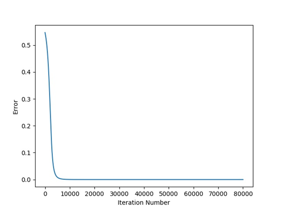
The next figure shows how the error changes by iteration which is also identical to what was presented for the previous implementation.

After making sure the code works correctly, next is to use a different number of hidden neurons. The only change required is to specify the desired number of hidden neurons in the network_architecture variable. The next code uses 8 hidden neurons.

import numpy
import matplotlib.pyplot

def sigmoid(sop):
    return 1.0/(1+numpy.exp(-1*sop))

def error(predicted, target):
    return numpy.power(predicted-target, 2)

def error_predicted_deriv(predicted, target):
    return 2*(predicted-target)

def sigmoid_sop_deriv(sop):
    return sigmoid(sop)*(1.0-sigmoid(sop))

def sop_w_deriv(x):
    return x

def update_w(w, grad, learning_rate):
    return w - learning_rate*grad

x = numpy.array([0.1, 0.4, 4.1])
target = numpy.array([0.2])

learning_rate = 0.001

# Number of inputs, number of neurons per each hidden layer, number of output neurons
network_architecture = numpy.array([x.shape[0], 8, 1])

# Initializing the weights of the entire network
w = []
w_temp = []
for layer_counter in numpy.arange(network_architecture.shape[0]-1):
    for neuron_nounter in numpy.arange(network_architecture[layer_counter+1]):
        w_temp.append(numpy.random.rand(network_architecture[layer_counter]))
    w.append(numpy.array(w_temp))
    w_temp = []
w = numpy.array(w)
w_old = w
print("Initial W : ", w)

for k in range(80000):
    # Forward Pass
    # Hidden Layer Calculations
    sop_hidden = numpy.matmul(w[0], x)

    sig_hidden = sigmoid(sop_hidden)

    # Output Layer Calculations
    sop_output = numpy.sum(w[1][0]*sig_hidden)

    predicted = sigmoid(sop_output)
    err = error(predicted, target)

    # Backward Pass
    g1 = error_predicted_deriv(predicted, target)

    ### Working with weights between hidden and output layer
    g2 = sigmoid_sop_deriv(sop_output)
    g3 = sop_w_deriv(sig_hidden)
    grad_hidden_output = g3*g2*g1
    w[1][0] = update_w(w[1][0], grad_hidden_output, learning_rate)
    
    ### Working with weights between input and hidden layer
    g5 = sop_w_deriv(x)
    for neuron_idx in numpy.arange(w[0].shape[0]):
        g3 = sop_w_deriv(w_old[1][0][neuron_idx])
        g4 = sigmoid_sop_deriv(sop_hidden[neuron_idx])
        grad_hidden_input = g5*g4*g3*g2*g1
        w[0][neuron_idx] = update_w(w[0][neuron_idx], grad_hidden_input, learning_rate)

    w_old = w
    print(predicted)

The next figure shows the relationship between the predicted output and the iteration number which proves that the GD algorithm is able to train the ANN successfully.

The relationship between the error and the iteration number is given in the next figure.

Conclusion

By the end of this part of the series, we have successfully implemented the GD algorithm to work with a variable number of hidden neurons within just a single hidden layer. It can also accept a variable number of inputs. In the next part, the implementation will be extended to allow the GD algorithm to work with more than 1 hidden layer.