Bring this project to life
The term 'pooling' would sound familiar to anyone conversant with Convolutional Neural Networks as it is a process commonly used after each convolution layer. In this article, we will be exploring the whys and the hows behind this fundamental process in CNN architectures.
The Pooling Process
Similar to convolution, the pooling process also utilizes a filter/kernel, albeit one without any elements (sort of an empty array). It essentially involves sliding this filter over sequential patches of the image and processing pixels caught in the kernel in some kind of way; basically the same as a convolution operation.
Strides In Computer Vision
In deep learning frameworks, there exists a not too popular, yet highly fundamental, parameter which dictates the behavior of convolution and pooling classes. In a more general sense, it controls the behavior of any class which employs a sliding window for one reason or the other. That parameter is termed 'stride.' It is referred to as the sliding window because scanning over an image with a filter resembles sliding a small window over the image's pixels).
The stride parameter determines how mxuch a filter is shifted in either dimension when performing sliding window operations like convolution and pooling.
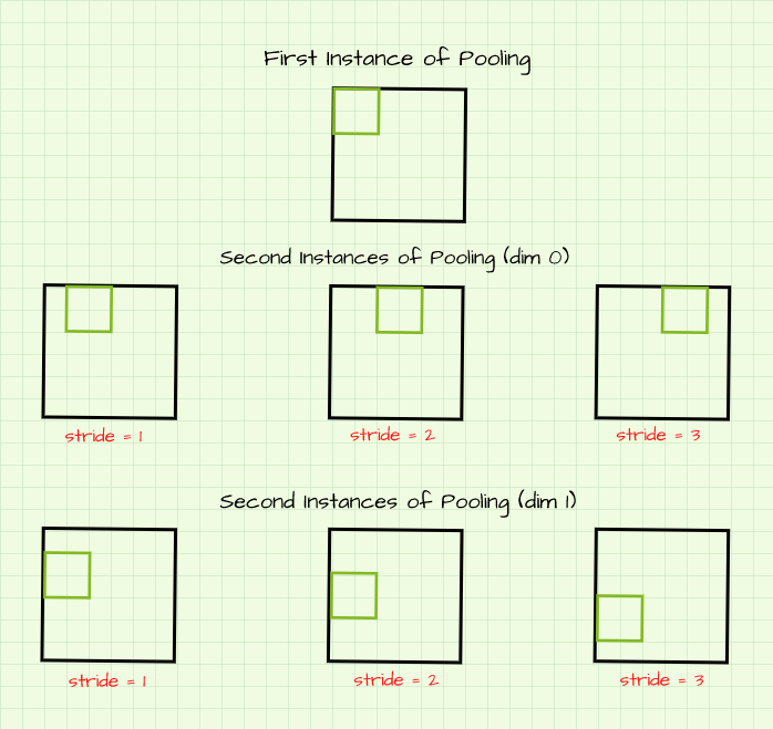
In the image above, filters are slid in both dim 0 (horizontal) and dim 1 (vertical) on the (6, 6) image. When stride=1, the filter is slid by one pixel. However, when stride=2 the filter is slid by two pixels; three pixels when stride=3. This has an interesting effect when generating a new image via a sliding window process; as a stride of 2 in both dimensions essentially generates an image which is half the size of its original image. Likewise a stride of 3 will produce an image which is a third of the size of its reference image and so on.
When stride > 1, a representation which is a fraction of the size of its reference image is produced.
When performing pooling operations, it is important to note that stride is always equal to the size of the filter by default. For instance, if a (2, 2) filter is to be used, stride is defaulted to a value of 2.
Types of Pooling
There are mainly two types of pooling operations used in CNNs, they are, Max Pooling and Average Pooling. The global variants of these two pooling operations also exist, but they are outside the scope of this particular article (Global Max Pooling and Global Average Pooling).
Max Pooling
Max pooling entails scanning over an image using a filter and at each instance returning the maximum pixel value caught within the filter as a pixel of its own in a new image.
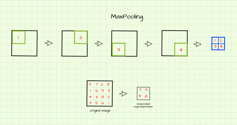
From the illustration, an empty (2, 2) filter is slid over a (4, 4) image with a stride of 2 as discussed in the section above. The maximum pixel value at every instance is returned as a distinct pixel of its own to form a new image. The resulting image is said to be a max pooled representation of the original image (Note that the resulting image is half the size of the original image due to a default stride of 2 as discussed in the previous section).
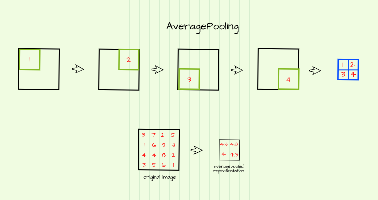
Average Pooling
Just like Max Pooling, an empty filter is also slid over the image but in this case the average/mean value of all the pixels caught in the filter is returned to form an average pooled representation of the original image as illustrated below.
Max Pooling Vs Average Pooling
From the illustrations in the previous section, one can clearly see that pixel values are much larger in the max pooled representation compared to the average pooled representation. In more simple terms, this simply means that representations resulting from max pooling are often sharper than those derived from average pooling.
Essence of Pooling
In one of my prior articles, I mentioned how Convolutional Neural Networks extract features as edges from an image via the process of convolution. These extracted features are termed feature maps. Pooling then acts on these feature maps and serves as a kind of principal component analysis (permit me to be quite liberal with that concept) by looking through the feature maps and producing a small sized summary in a process called down-sampling.
In less technical terms, pooling generates small sized images which retain all the essential attributes (pixels) of a reference image. Basically, one could produce a (25, 25) pixel image of a car which would retain all the general details and makeup of a reference image sized (400, 400) by iteratively pooling 4 times using a (2, 2) kernel. It does this by utilizing strides which are greater than 1, allowing for the production of representations which are a fraction of the original image.
Going back to CNNs, as convolution layers get deeper, the number of feature maps (representations resulting from convolution) increase. If the feature maps are of the same size as the image provided to the network, computation speed would be severely hampered due to the large volume of data present in the network particularly during training. By progressively down-sampling these feature maps, the amount of data in the network is effectively kept in check even as feature maps increase in number. What this means is that the network will progressively have reasonable amounts of data to deal with without losing any of the essential features extracted by the previous convolution layer resulting in faster compute.
Another effect of pooling is that it allows Convolutional Neural Networks to be more robust as they become translation invariant. This means the network will be able to extract features from an object of interest regardless of the object's position in an image (more on this in a future article).
Under The Hood.
Bring this project to life
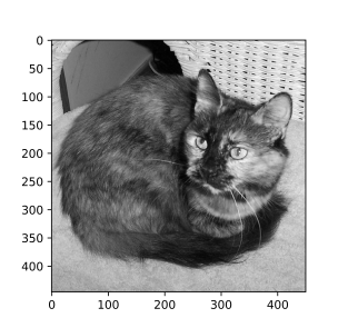
In this section we will be using a manually written pooling functions in a bid to visualize the pooling process so as to better understand what actually goes on. Two functions are provided, one for max pooling and the other for average pooling. Using the functions, we will be attempting to pool the image of size (446, 550) pixels below.
#  import these dependencies
import torch
import numpy as np
import matplotlib.pyplot as plt
import torch.nn.functional as F
from tqdm import tqdmMax Pooling Behind The Scenes
def max_pool(image_path, kernel_size=2, visualize=False, title=''):
      """
      This function replicates the maxpooling
      process
      """

      #  assessing image parameter
      if type(image_path) is np.ndarray and len(image_path.shape)==2:
        image = image_path
      else:
        image = cv2.imread(image_path, cv2.IMREAD_GRAYSCALE)

      #  creating an empty list to store convolutions
      pooled = np.zeros((image.shape[0]//kernel_size,
                        image.shape[1]//kernel_size))

      #  instantiating counter
      k=-1
      #  maxpooling
      for i in tqdm(range(0, image.shape[0], kernel_size)):
        k+=1
        l=-1
        if k==pooled.shape[0]:
          break
        for j in range(0, image.shape[1], kernel_size):
          l+=1
          if l==pooled.shape[1]:
            break
          try:
            pooled[k,l] = (image[i:(i+kernel_size),
                                j:(j+kernel_size)]).max()
          except ValueError:
            pass

      if visualize:
        #  displaying results
        figure, axes = plt.subplots(1,2, dpi=120)
        plt.suptitle(title)
        axes[0].imshow(image, cmap='gray')
        axes[0].set_title('reference image')
        axes[1].imshow(pooled, cmap='gray')
        axes[1].set_title('maxpooled')
return pooledThe function above replicates the max pooling process. Using the function, let's attempt to max pool the reference image using a (2, 2) kernel.
max_pool('image.jpg', 2, visualize=True)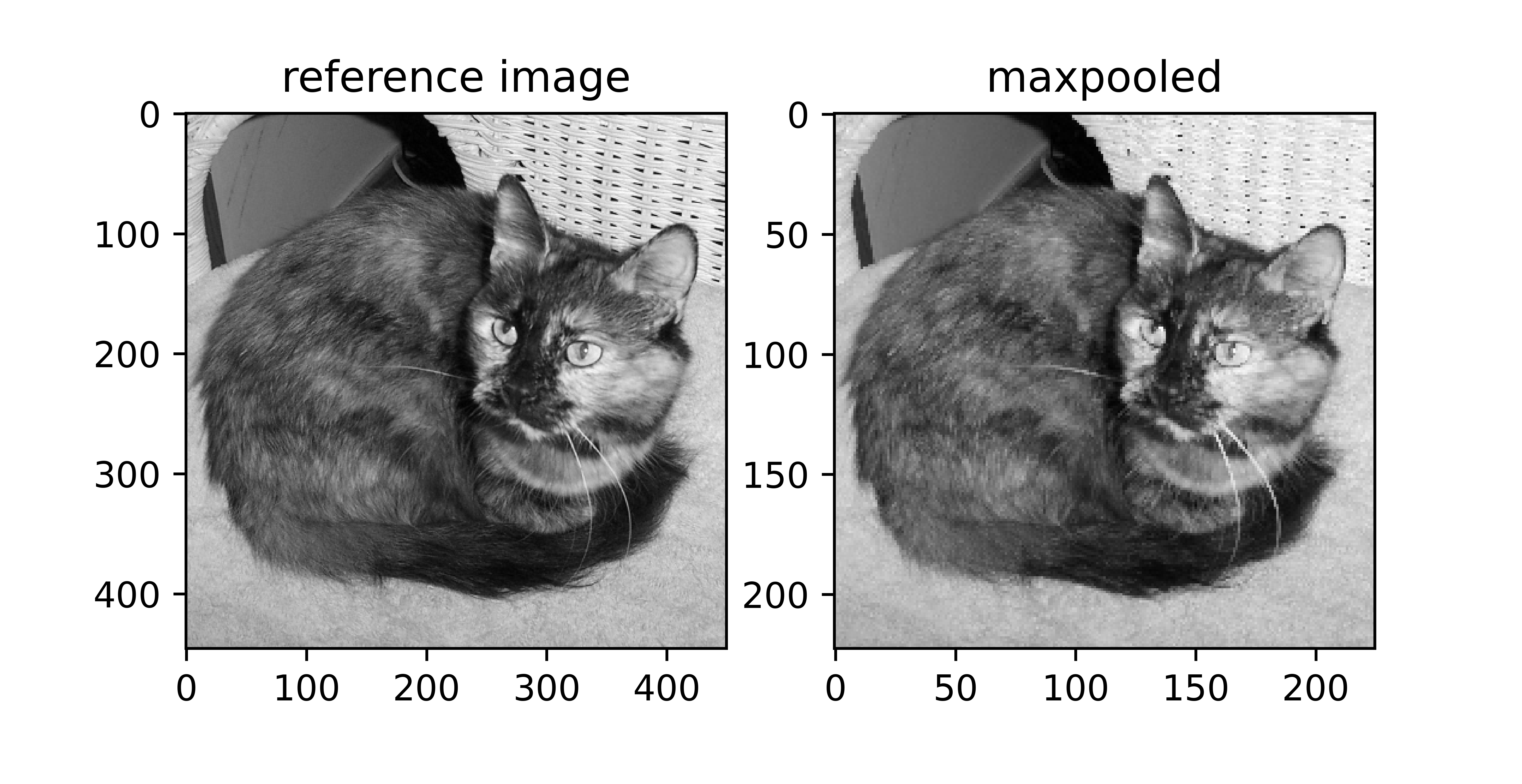
Looking at the number-lines on each axis it is clear to see that the image has reduced in size but has kept all of its details intact. Its almost like the process has extracted the most salient pixels and produced a summarized representation which is half the size of the reference image (half because a (2, 2) kernel was used).
The function below allows for the visualization of several iterations of the max pooling process.
def visualize_pooling(image_path, iterations, kernel=2):
      """
      This function helps to visualise several
      iterations of the pooling process
      """
      image = cv2.imread(image_path, cv2.IMREAD_GRAYSCALE)

      #  creating empty list to hold pools
      pools = []
      pools.append(image)

      #  performing pooling
      for iteration in range(iterations):
        pool = max_pool(pools[-1], kernel)
        pools.append(pool)

      #  visualisation
      fig, axis = plt.subplots(1, len(pools), dpi=700)
      for i in range(len(pools)):
        axis[i].imshow(pools[i], cmap='gray')
        axis[i].set_title(f'{pools[i].shape}', fontsize=5)
        axis[i].axis('off')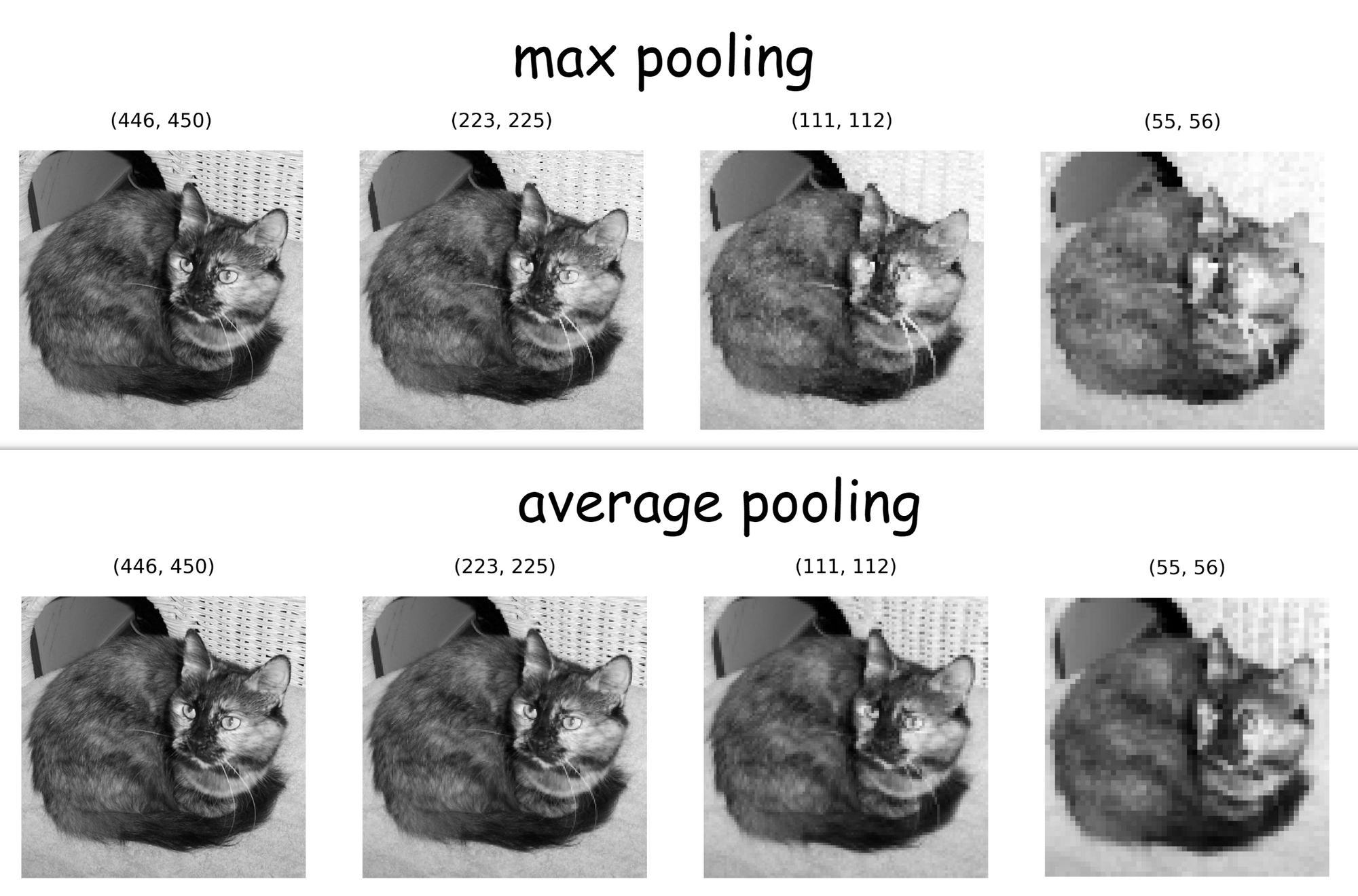
passUsing this function we can visualize 3 generations of max pooled representation using a (2, 2) filter as seen below. The image goes from a size of (446, 450) pixels to a size of (55, 56) pixels (essentially a 1.5% summary), whilst maintaining its general makeup.
visualize_pooling('image.jpg', 3)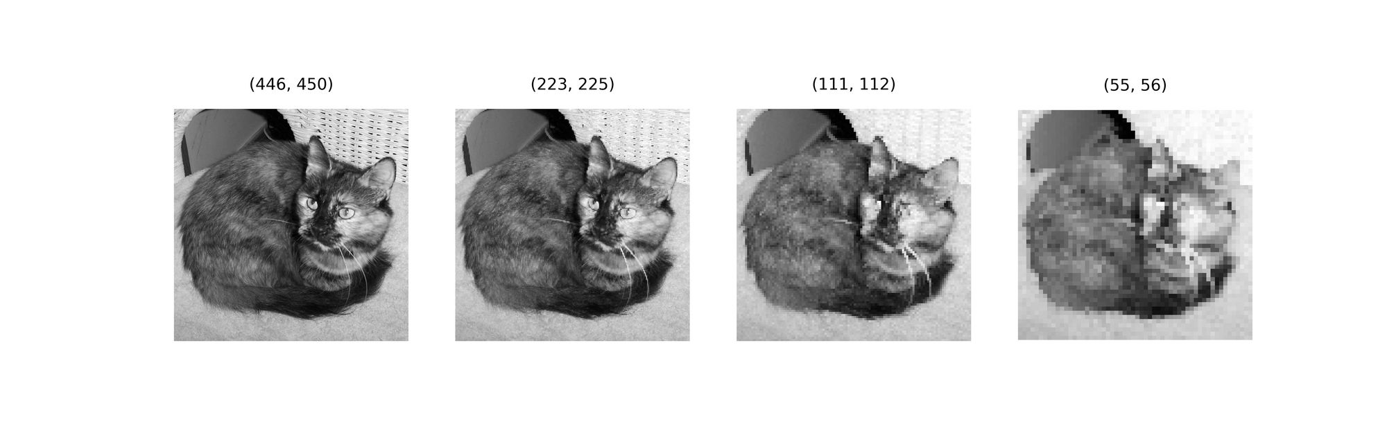
The effects of using a larger kernel (3, 3) are seen below, as expected the reference image reduces to 1/3 its preceding size for every iteration. By the 3rd iteration, a pixelated (16, 16) down-sampled representation is produced (a 0.1% summary). Although pixelated, the overall idea of the image is somewhat still maintained.
visualize_pooling('image.jpg', 3, kernel=3)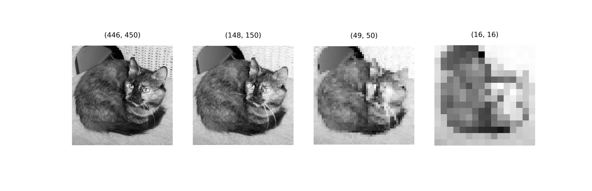
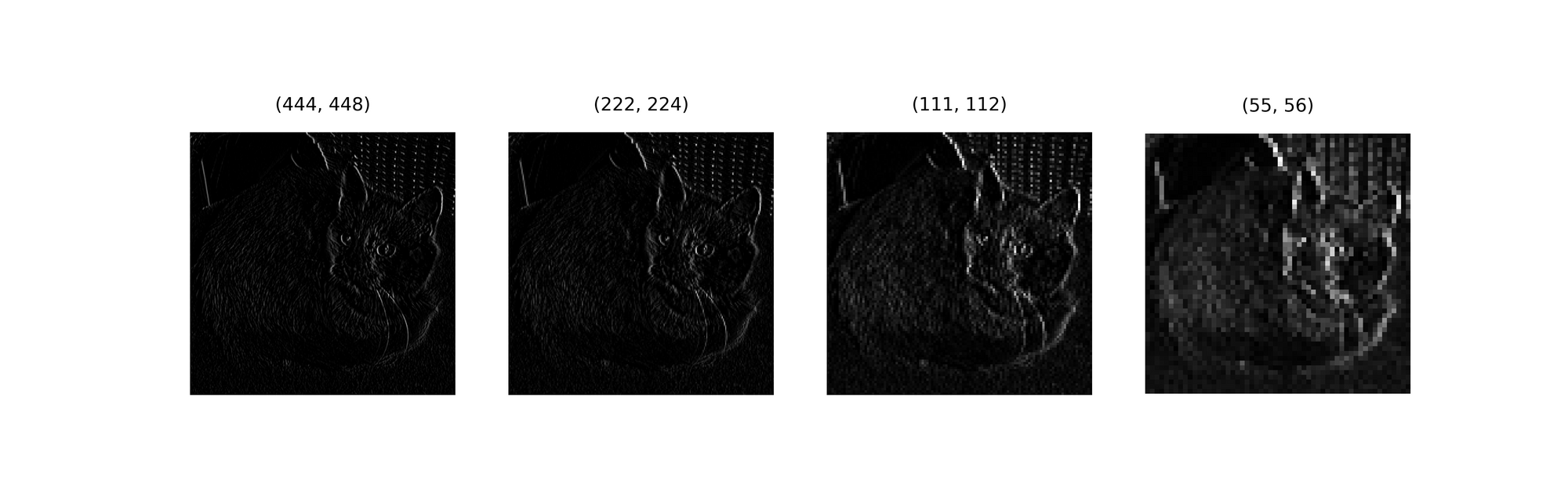
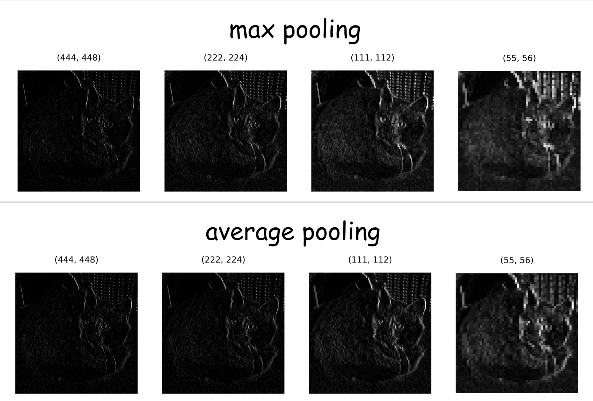
To properly try to imitate what the max pooling process might look like in a Convolutional Neural Network, let's run a couple of iterations over vertical edges detected in the image using a Prewitt operator.
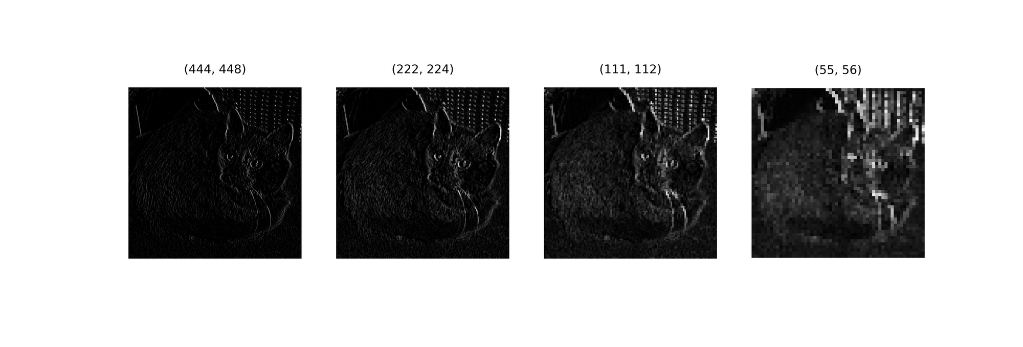
By the third iteration, although the image had reduced in size, it can be seen that its features (edges) have been brought progressively into focus.
Average Pooling Behind The Scenes
def average_pool(image_path, kernel_size=2, visualize=False, title=''):
      """
      This function replicates the averagepooling
      process
      """

      #  assessing image parameter
      if type(image_path) is np.ndarray and len(image_path.shape)==2:
        image = image_path
      else:
        image = cv2.imread(image_path, cv2.IMREAD_GRAYSCALE)

      #  creating an empty list to store convolutions
      pooled = np.zeros((image.shape[0]//kernel_size,
                        image.shape[1]//kernel_size))

      #  instantiating counter
      k=-1
      #  averagepooling
      for i in tqdm(range(0, image.shape[0], kernel_size)):
        k+=1
        l=-1
        if k==pooled.shape[0]:
          break
        for j in range(0, image.shape[1], kernel_size):
          l+=1
          if l==pooled.shape[1]:
            break
          try:
            pooled[k,l] = (image[i:(i+kernel_size),
                                j:(j+kernel_size)]).mean()
          except ValueError:
            pass

      if visualize:
        #  displaying results
        figure, axes = plt.subplots(1,2, dpi=120)
        plt.suptitle(title)
        axes[0].imshow(image, cmap='gray')
        axes[0].set_title('reference image')
        axes[1].imshow(pooled, cmap='gray')
        axes[1].set_title('averagepooled')
return pooledThe function above replicates the average pooling process. Note that this is identical code to the max pooling function with the distinction of using the mean() method as the kernel is slid over the image. An average pooled representation of our reference image is visualized below.
average_pool('image.jpg', 2, visualize=True)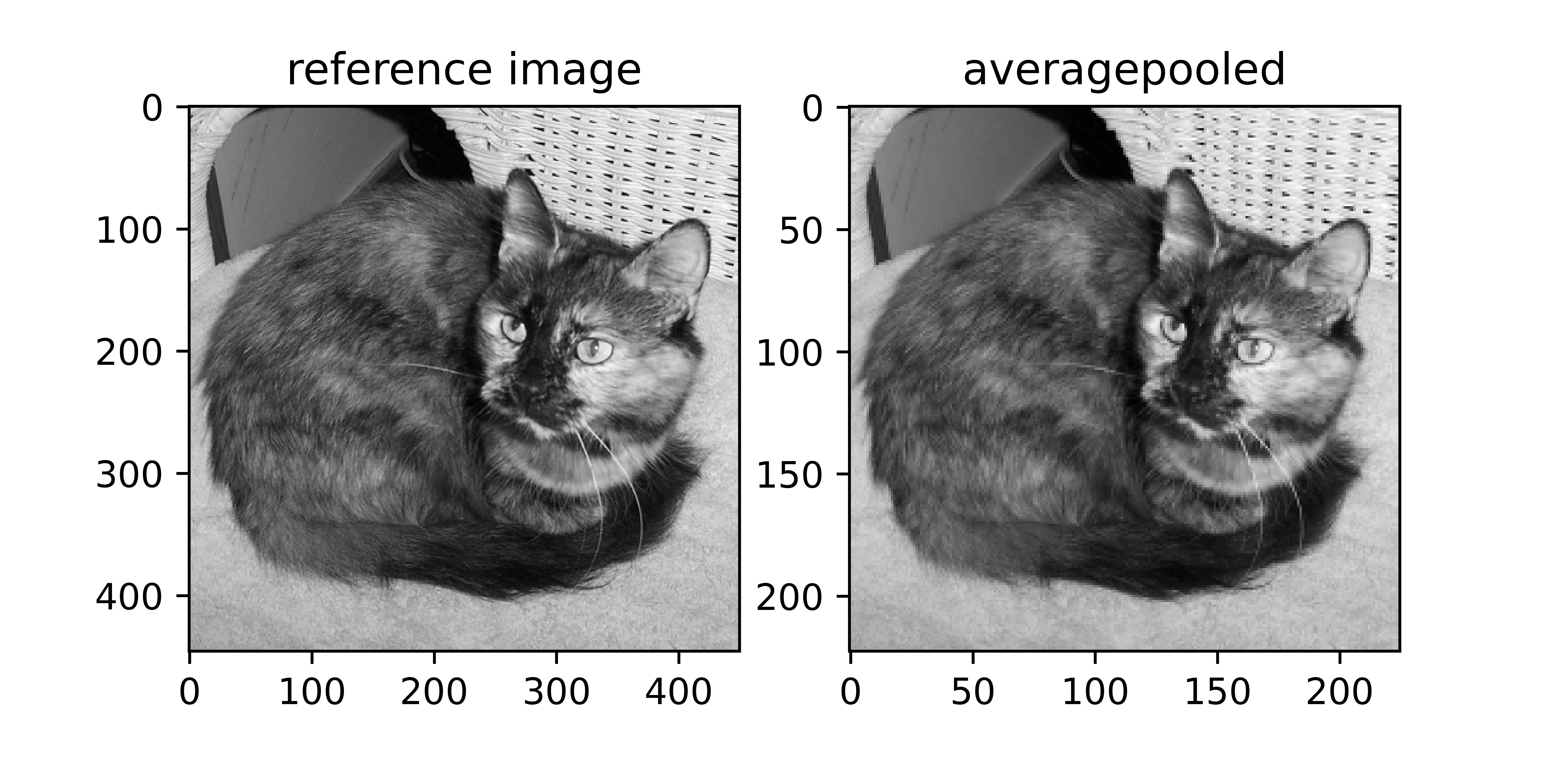
Similar to max pooling, it can be seen that the image has been reduced to half its size whilst keeping its most important attributes. This is quite interesting because unlike max pooling, average pooling does not directly use the pixels in the reference image, rather it combines them basically creating new attributes (pixels), and yet details in the reference image are preserved.
Let's see how the average pooling process progresses through 3 iterations using the visualization function below.
def visualize_pooling(image_path, iterations, kernel=2):
      """
      This function helps to visualise several
      iterations of the pooling process
      """
      image = cv2.imread(image_path, cv2.IMREAD_GRAYSCALE)

      #  creating empty list to hold pools
      pools = []
      pools.append(image)

      #  performing pooling
      for iteration in range(iterations):
        pool = average_pool(pools[-1], kernel)
        pools.append(pool)

      #  visualisation
      fig, axis = plt.subplots(1, len(pools), dpi=700)
      for i in range(len(pools)):
        axis[i].imshow(pools[i], cmap='gray')
        axis[i].set_title(f'{pools[i].shape}', fontsize=5)
        axis[i].axis('off')
passAgain, even as the image size progressively reduces by half after each iteration, its details remains albeit with gradual pixelation (as expected in small sized images).
visualize_pooling('image.jpg', 3)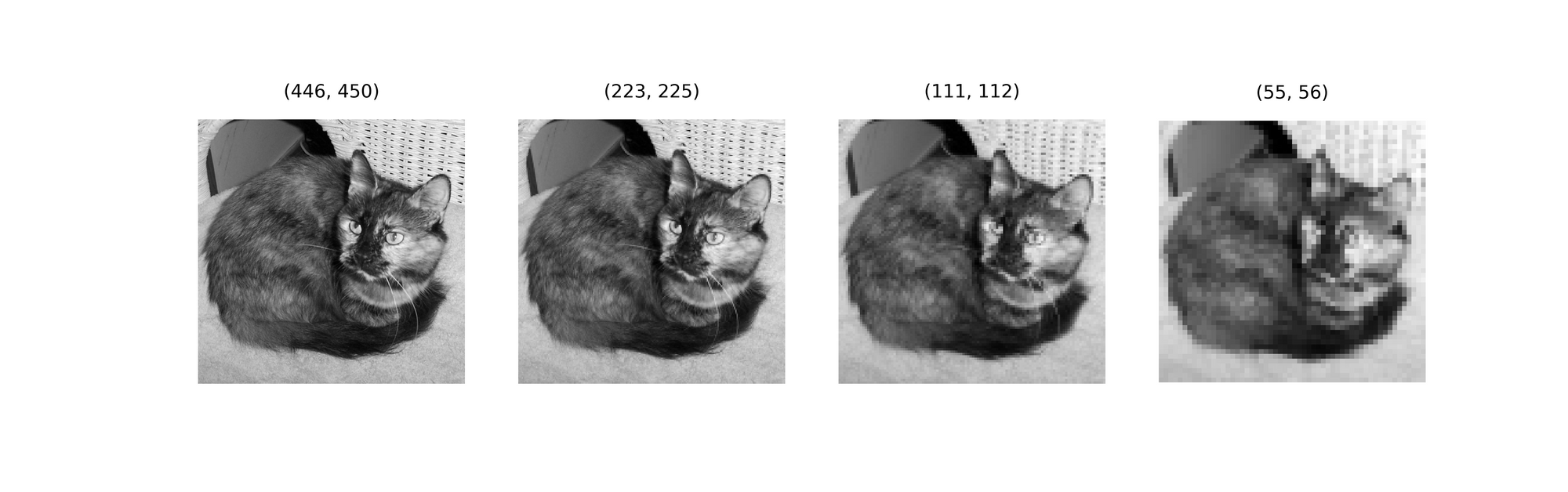
Average pooling using a (3, 3) kernel yields the following result. As expected, image size is reduced to 1/3 of its preceding value. Heavy pixelation sets in by the 3 iteration just like in max pooling but the overall attributes of the image are reasonably intact.
visualize_pooling('image.jpg', 3, kernel=3)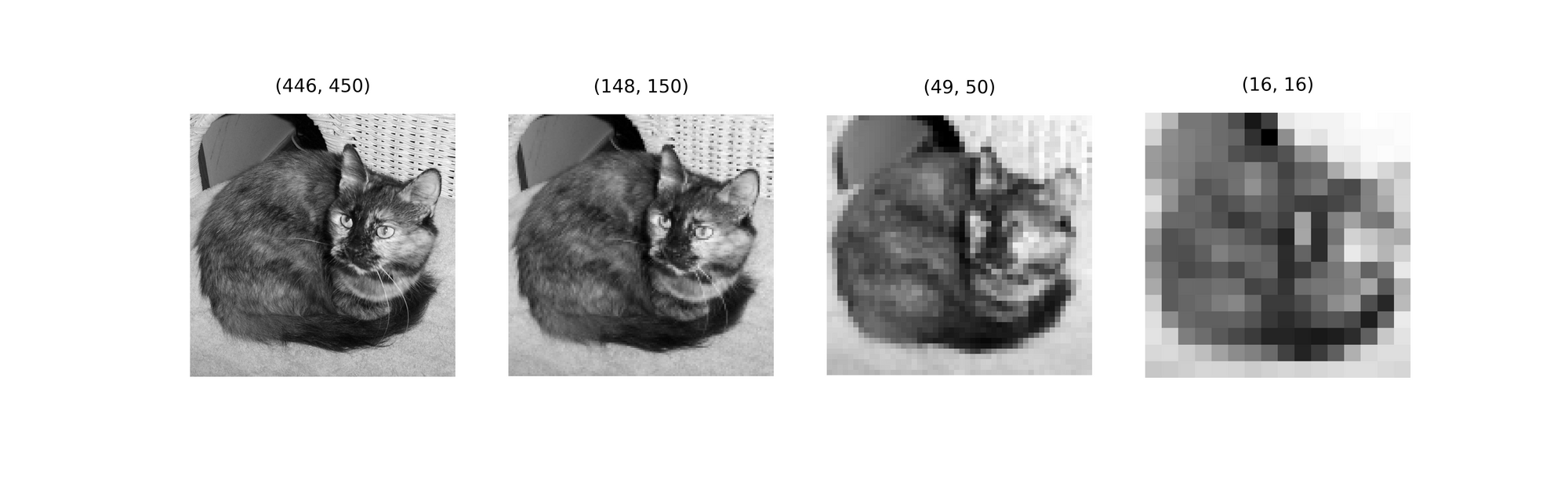
Running (2, 2) average pooling over vertical edges detected using a Prewitt operator produces the results below. Just as in max pooling, the image features (edges) become more pronounced with progressive average pooling.
Max Pooling or Average Pooling?
A natural response after learning about both the max and average pooling processes is to wonder which of them is more superior for computer vision applications. The truth is, arguments can be made either way.
On one hand, since max pooling selects the highest pixel values caught in a kernel, it produces a much sharper representation.
In a Convolutional Neural Network context, that means it does a much better job at bringing detected edges into focus in feature maps as seen in the image below.
On the other hand, an argument could be made in favor of average pooling that it produces more generalized feature maps. Consider our reference image of size (444, 448), when pooling with a kernel of size (2, 2) its pooled representation is of a size (222, 224), basically 25% of the total pixels in the reference image. Because max pooling basically selects pixels, some argue that it results in a loss of data which might be detrimental to the network's performance. In opposing fashion, instead of selecting pixels, average pooling combines pixels into one by computing their mean value, therefore some are of the belief that average pooling simply compresses pixels by 75% instead of explicitly removing the which would yield more generalized feature maps thereby doing a better job at combating overfitting.
What side of the divide do I belong? Personally I believe max pooling's ability to further highlight edges in feature maps gives it an edge in computer vision/deep learning applications hence why it is more popular. This is not to say that the use of average pooling will severely degrade network performance however, just a personal opinion.
Final Remarks
In this article we've developed an intuition of what pooling entails in the context of Convolutional Neural Networks. We've looked at two main types of pooling and the difference in the pooled representations produced by each one.
For all the talk about pooling in CNNs, bear in mind that most architectures these days tend to favor strided convolution layers over pooling layers for down-sampling as they reduce the network's complexity. Regardless, pooling remains an essential component of Convolutional Neural Networks.