Vectorization and Broadcasting with Pytorch

The performance gains derived from running your machine learning code on a GPU can be huge. But GPUs are optimized for code that needs to perform the same operation, thousands of times, in parallel. Therefore, it's important that we write our code that way too.

Earlier this week I was training some word embeddings. Recall that word embeddings are dense vectors that are supposed to capture word meaning, and the distance (cosine distance, or euclidean distance) between two word embeddings should be smaller if the words are similar in meaning.

I wanted to evaluate the quality of my trained word embeddings by evaluating them against a word similarity dataset, like the Stanford Rare Word Similarity dataset. Word similarity datasets collect human judgments about the distance between words. A word similarity dataset for a vocabulary, V, can be represented as a |V| x |V| matrix, S, where S[i][j] represents the similarity between words V[i] and V[j].

I needed to write some Pytorch code that would compute the cosine similarity between every pair of embeddings, thereby producing a word embedding similarity matrix that I could compare against S.

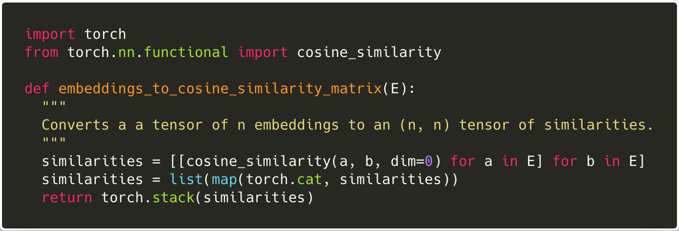
Here is my first attempt:

source

We loop through the embeddings matrix E, and we compute the cosine similarity for every pair of embeddings, a and b. This gives us a list of lists of floats. We then use torch.cat to convert each sublist into a tensor, and then we torch.stack the entire list into a single 2D (n x n) tensor.

Okay, so let's see how this loopy code performs! We'll generate a random matrix of 20,000 1oo-dimentional word embeddings, and compute the cosine similarity matrix.

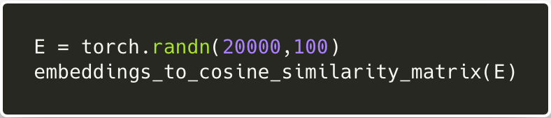
We're running this benchmark on one of PaperSpace's powerful P6000 machines, but a quick glance at the output of nvidia-smi shows GPU-utilization at 0%, and top shows that the CPU is hard at work. It is 5 hours before the program terminates.

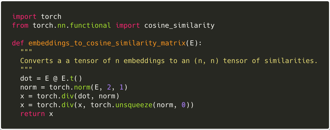
Now, we rewrite the function in vectorized form:

source

A quick performance test on the P6000 shows that this function takes only 3.779 seconds to compute a similarity matrix from 20,000 100-dimensional embeddings!

Let's walk through the code. The key idea is that we are breaking down the cosine_similarity function into its component operations, so that we can parallelize the 10,000 computations instead of doing them sequentially.

The cosine_similarity of two vectors is just the cosine of the angle between them:

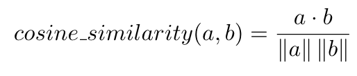
1. First, we matrix multiply E with its transpose.
   
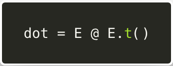
   This results in a (num_embeddings, num_embeddings) matrix, dot. If you think about how matrix multiplication works (multiply and then sum), you'll realize that each dot[i][j] now stores the dot product of E[i] and E[j].

2. Then, we compute the magnitude of each embedding vector.
   
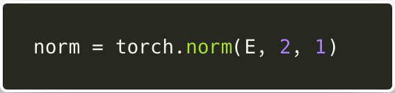
   The 2 denotes that we are computing the L-2 (euclidean) norm of each vector. The 1 tells Pytorch that our embeddings matrix is laid out as (num_embeddings, vector_dimension) and not (vector_dimension, num_embeddings).
   norm is now a row vector, where norm[i] = ||E[i]||.

3. We divide each (E[i] dot E[j]) by ||E[j]||.
   
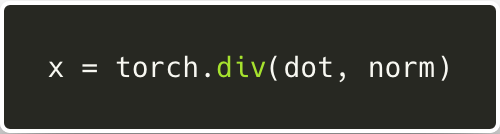
   Here, we're exploiting something called broadcasting. Notice that we're dividing a matrix (num_embeddings, num_embeddings) by a row vector (num_embeddings,). Without allocating more memory Pytorch will broadcast the row vector down, so that we can imagine we are dividing by a matrix, made up of num_embeddings rows, each containing the original row vector. The result is that each cell in our original matrix has now been divided by ||E[j]||, the magnitude of the embedding corresponding to its column-number.

4. Finally, we divide by ||E[i]||:
   
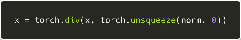
   Again, we're using broadcasting, but this time we're converting norm into a column vector first, so that broadcasting will copy columns instead of rows. The result is that each cell, x[i][j], is divided by ||E[i]||, the magnitude of the i-th embedding.

That's it! We've computed a matrix containing the pair-wise cosine similarity between every pair of embeddings, and derived massive performance gains from vectorization and broadcasting!

Conclusion
Next time you're wondering why your machine learning code is running slowly, even on a GPU, consider vectorizing any loopy code!

If you'd like to read more about the things we touched on in this blog post, check out some of these links:

• Pytorch Broadcasting Semantics
• Learning Word Embeddings with Word2Vec
• Problems With Evaluation of Word Embeddings Using Word Similarity Tasks