Attention Mechanisms in Recurrent Neural Networks (RNNs) With Keras

In this tutorial, we’ll cover attention mechanisms in RNNs: how they work, the network architecture, their applications, and how to implement attention mechanism-imbued RNNs using Keras.

Specifically, we'll cover:

• The Problem With Sequence-to-Sequence Models for Neural Machine Translation
• An Introduction to Attention Mechanisms
• Categories of Attention Mechanisms
• Applications of Attention Mechanisms
• Neural Machine Translation Using an RNN With Attention Mechanism (Keras)
• Conclusion

You can run all of the code in this tutorial on a free GPU from a Gradient Community Notebook.

Let’s get started!

Note: All of the examples in this series (Advanced RNNs) have been trained on TensorFlow 2.x.

The Problem With Sequence-to-Sequence Models for Neural Machine Translation

The machine translation problem has thrust us towards inventing the “Attention Mechanism”. Machine translation is the automatic conversion from one language to another. The conversion has to happen using a computer program, where the program has to have the intelligence to convert the text from one language to the other. When a neural network performs this job, it’s called “Neural Machine Translation”.

Machine translation is one of the most challenging problems in artificial intelligence due to the ambiguity and complexity involved in human language (be it any).

Despite the complexity, we’ve seen many approaches arise to solve this problem.

Neural networks played a crucial role in devising ways to automate the machine translation process. The first neural network seen as suitable for this application was a sequence-to-sequence model.

As seen in Introduction to Encoder-Decoder Sequence-to-Sequence Models (Seq2Seq), a sequence-to-sequence model comprises an encoder and a decoder, wherein an encoder produces a context vector (encoded representation) as a by-product. This vector is given to a decoder which then starts generating the output.

Interestingly, this is how the usual translation process happens.

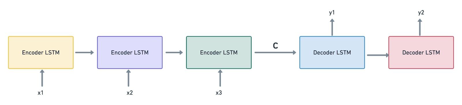
The encoder-decoder sequence-to-sequence model in itself is similar to the current translation process. It involves encoding the source language into a suitable representation, and then decoding it into a target language where the input and output vectors needn’t be of the same size. However, this model has its share of problems:

• The context vector is of a fixed length. Assume that there’s a long sequence that has to be encoded. Owing to the encoded vector’s constant size, it can get difficult for the network to define an encoded representation for long sequences. Oftentimes, it may forget the earlier parts of the sequence, leading to the loss of vital information.
• A sequence-to-sequence model considers the encoder’s final state as the context vector to be passed on to the decoder. In other words, it doesn’t examine the intermediate states generated during the encoding process. This can also contribute to the loss of information if there are long sequences of input data involved.

These two factors can act as the bottlenecks to improving the performance of a sequence-to-sequence model. To eradicate this issue, we can extend this architecture by enabling the model to soft-search the input to filter the relevant positions in it. It can then predict the output based on the relative context vectors and all the previously generated output words.

This is precisely what the attention mechanism does!

An Introduction to Attention Mechanisms

Going by the typical English vocabulary, “Attention” refers to directing your focus on something. If we consider the neural machine translation example, where do you think “Attention” fits in?

The attention mechanism aims to solve both of the issues we discussed when training a neural machine translation model with a sequence-to-sequence model. Firstly, when there’s attention integrated, the model need not compress the encoded output into a single context vector. Instead, it encodes the input sequence into a sequence of vectors and picks a subset of these vectors depending on the decoder’s hidden states. In a nutshell, there’s “attention” applied to choose what’s necessary, without letting go of other necessary information.

This is what an RNN model with an attention mechanism looks like:

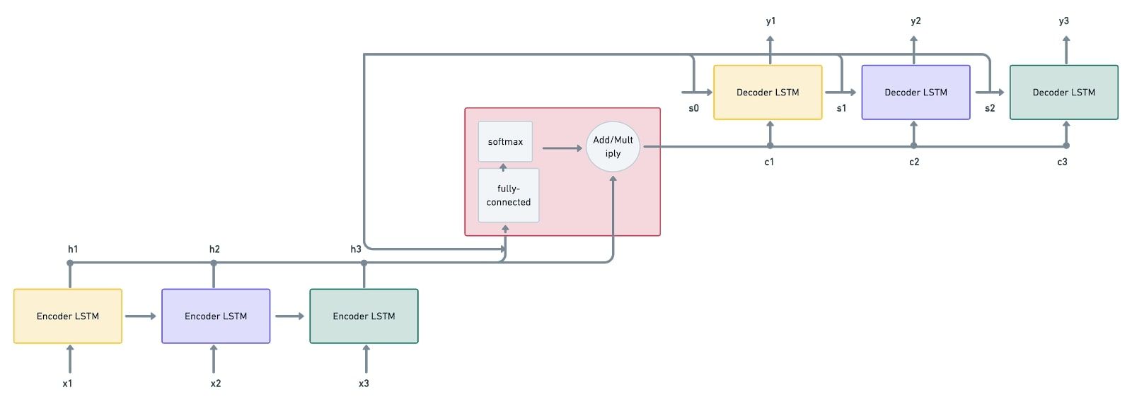
Here’s a step-by-step procedure as to how the machine translation problem is solved using the attention mechanism:

• Firstly, the input sequence $x_1, x_2, x_3$ is given to the encoder LSTM. The vectors $h_1, h_2, h_3$ are computed by the encoders from the given input sequence. These vectors are the inputs given to the attention mechanism. This is followed by the decoder inputting the first state vector $s_0$, which is also given as an input to the attention mechanism. We now have $s_0$ and $h_1, h_2, h_3$ as inputs.
• The attention mechanism mode (depicted in a red box) accepts the inputs and passes them through a fully-connected network and a softmax activation function, which generates the “attention weights”.
• The weighted sum of the encoder’s output vectors is then computed, resulting in a context vector $c_1$. Here, the vectors are scaled according to the attention weights.
• It’s now the decoder's job to process the state and context vectors to generate the output vector $y_1$.
• The decoder also produces the consequent state vector $s_1$, which is again given to the attention mechanism model along with the encoder’s outputs.
• This produces the weighted sum, resulting in the context vector $c_2$.
• This process continues until all the decoders have generated the output vectors $y_1, y_2, y_3$.

The catch in an attention mechanism model is that the context vectors enable the decoder to focus only on certain parts of its input (in fact, context vectors are generated from the encoder’s outputs). This way, the model stays attentive to all those inputs which it thinks are crucial in determining the output.

Categories of Attention Mechanisms

We can segregate attention mechanisms broadly into three categories: Self-Attention, Soft Attention, and Hard Attention mechanisms.

Self-Attention

Self-Attention helps the model to interact within itself. The long short-term memory-networks for machine reading paper uses self-attention. The learning process is depicted in the example below:

The attention here is computed within the same sequence. In other words, self-attention enables the input elements to interact among themselves.

Soft Attention

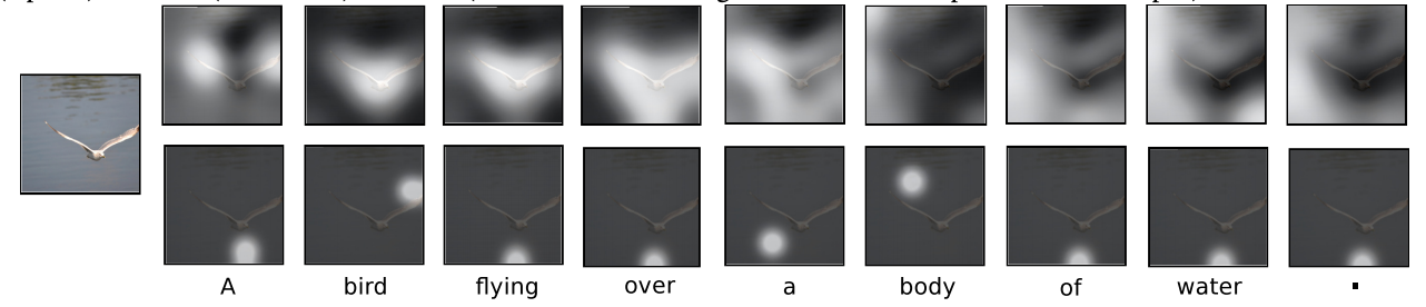
Soft attention ‘softly’ places the attention weights over all patches of the input (image/sentence), i.e., it employs the weighted average mechanism. It measures the attention concerning various chunks of the input, and outputs the weighted input features. It discredits the areas which are irrelevant to the task at hand by assigning them low weights. This way, soft attention doesn’t confine its focus to specific parts of the image or the sentence; instead, it learns continuously.

Soft attention is a fully differentiable attention mechanism, where the gradients can be propagated automatically during backpropagation.

Hard Attention

“Hard”, as the name suggests, focuses on only a specific part of the image/sentence. During backpropagation, to estimate the gradients for all the other states, we need to perform sampling and average the results using the Monte Carlo method.

Applications of Attention Mechanisms

Just a few applications of attention mechanisms include:

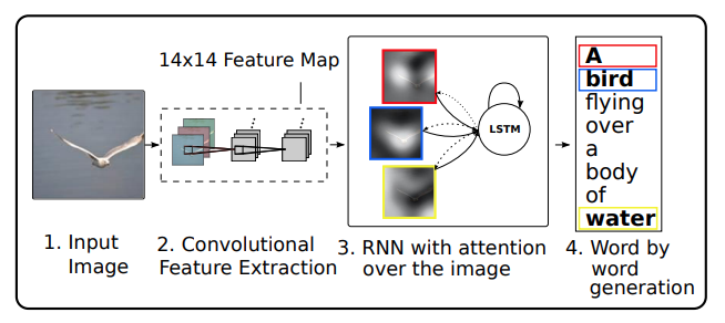
• Image Captioning
• Speech Recognition
• Machine Translation
• Self-Driving Cars
• Document Summarization

Neural Machine Translation Using an RNN With Attention Mechanism (Keras)

An RNN can be used to achieve machine translation. Generally, a simple RNN laced with an encoder-decoder sequence-to-sequence model does this job. However, as stated in the section ‘The Problem with Sequence-to-Sequence Models for Neural Machine Translation’, a crammed representation of the encoded output might ignore vital features required for the translation process. To eradicate this problem, when we embed the attention mechanism with an encoder-decoder sequence-to-sequence model, we do not have to compromise on the loss of information when there are long sequences of text involved.

The attention mechanism focuses on all those inputs which are really required for the output to be generated. There’s no compression involved; instead, it considers all the encoder’s outputs and assigns importance to them according to the decoder’s hidden states.

Here’s a step-by-step process to employ an RNN model (encoder-decoder sequence-to-sequence with attention mechanism) for French to English translation.

Don't forget that you can follow along with the code and run it on a free GPU from a Gradient Community Notebook.

Step 1: Import the Dataset

First, import the English-to-French dataset (download link). It has about 185,583 language translation pairs.  

Untar the dataset and store the txt file path.

# Untar the dataset
!unzip 'fra-eng.zip'

# Get the txt file which has English -> French translation
path_to_file = "fra.txt"

Step 2: Preprocess the Dataset

The dataset has Unicode characters, which have to be normalized.

Moreover, all the tokens in the sequences have to be cleaned using the regular expressions library.

Remove unwanted spaces, include a space between every word and the punctuation following it (to differentiate between both), replace unwanted characters with spaces, and append <start> and <end> tokens to specify the start and end of a sequence.

Encapsulate the unicode conversion in a function unicode_to_ascii() and sequence preprocessing in a function preprocess_sentence().

import unicodedata

import re

# Convert the unicode sequence to ascii
def unicode_to_ascii(s):

  # Normalize the unicode string and remove the non-spacking mark
  return ''.join(c for c in unicodedata.normalize('NFD', s)
      if unicodedata.category(c) != 'Mn')

# Preprocess the sequence
def preprocess_sentence(w):

  # Clean the sequence
  w = unicode_to_ascii(w.lower().strip())

  # Create a space between word and the punctuation following it
  w = re.sub(r"([?.!,¿])", r" \1 ", w)
  w = re.sub(r'[" "]+', " ", w)

  # Replace everything with space except (a-z, A-Z, ".", "?", "!", ",")
  w = re.sub(r"[^a-zA-Z?.!,¿]+", " ", w)

  w = w.strip()

  # Add a start and stop token to detect the start and end of the sequence
  w = '<start> ' + w + ' <end>'
  return w

Step 3: Prepare the Dataset

Next, prepare a dataset out of the raw data we have. Create word pairs combining the English sequences and their related French sequences.

import io

# Create the Dataset
def create_dataset(path, num_examples):
  lines = io.open(path, encoding='UTF-8').read().strip().split('\n')

  # Loop through lines (sequences) and extract the English and French sequences. Store them as a word-pair
  word_pairs = [[preprocess_sentence(w) for w in l.split('\t', 2)[:-1]]  for l in lines[:num_examples]]
  return zip(*word_pairs)

Check if the dataset has been created properly.

en, fra = create_dataset(path_to_file, None)
print(en[-1])
print(fra[-1])

# Output
<start> if someone who doesn t know your background says that you sound like a native speaker , it means they probably noticed something about your speaking that made them realize you weren t a native speaker . in other words , you don t really sound like a native speaker . <end>
<start> si quelqu un qui ne connait pas vos antecedents dit que vous parlez comme un locuteur natif , cela veut dire qu il a probablement remarque quelque chose a propos de votre elocution qui lui a fait prendre conscience que vous n etes pas un locuteur natif . en d autres termes , vous ne parlez pas vraiment comme un locuteur natif . <end>

Now tokenize the sequences. Tokenization is the mechanism of creating an internal vocabulary comprising English and French tokens (i.e. words), converting the tokens (or, in general, sequences) to integers, and padding them all to make the sequences possess the same length. All in all, tokenization facilitates the model training process.

Create a function tokenize() to encapsulate all the above-mentioned requirements.

import tensorflow as tf

# Convert sequences to tokenizers
def tokenize(lang):
  lang_tokenizer = tf.keras.preprocessing.text.Tokenizer(
      filters='')
  
  # Convert sequences into internal vocab
  lang_tokenizer.fit_on_texts(lang)

  # Convert internal vocab to numbers
  tensor = lang_tokenizer.texts_to_sequences(lang)

  # Pad the tensors to assign equal length to all the sequences
  tensor = tf.keras.preprocessing.sequence.pad_sequences(tensor,
                                                         padding='post')

  return tensor, lang_tokenizer

Load the tokenized dataset by calling the create_dataset() and tokenize() functions.

# Load the dataset
def load_dataset(path, num_examples=None):
 
  # Create dataset (targ_lan = English, inp_lang = French)
  targ_lang, inp_lang = create_dataset(path, num_examples)

  # Tokenize the sequences
  input_tensor, inp_lang_tokenizer = tokenize(inp_lang)
  target_tensor, targ_lang_tokenizer = tokenize(targ_lang)

  return input_tensor, target_tensor, inp_lang_tokenizer, targ_lang_tokenizer

Reduce the number of data samples required to train the model. Employing the whole dataset will consume a lot more time for training the model.

# Consider 50k examples
num_examples = 50000
input_tensor, target_tensor, inp_lang, targ_lang = load_dataset(path_to_file, num_examples)

# Calculate max_length of the target tensors
max_length_targ, max_length_inp = target_tensor.shape[1], input_tensor.shape[1]

The max_length of both the input and target tensors is essential to determine every sequence's maximum padded length.

Step 4: Create the Dataset

Segregate the train and validation datasets.

!pip3 install sklearn

from sklearn.model_selection import train_test_split

# Create training and validation sets using an 80/20 split
input_tensor_train, input_tensor_val, target_tensor_train, target_tensor_val = train_test_split(input_tensor, target_tensor, test_size=0.2)

print(len(input_tensor_train), len(target_tensor_train), len(input_tensor_val), len(target_tensor_val))

# Output
40000 40000 10000 10000

Validate the mapping that’s been created between the tokens of the sequences and the indices.

# Show the mapping b/w word index and language tokenizer
def convert(lang, tensor):
  for t in tensor:
    if t != 0:
      print ("%d ----> %s" % (t, lang.index_word[t]))
      
print ("Input Language; index to word mapping")
convert(inp_lang, input_tensor_train[0])
print ()
print ("Target Language; index to word mapping")
convert(targ_lang, target_tensor_train[0])

# Output
Input Language; index to word mapping
1 ----> <start>
140 ----> quel
408 ----> idiot
3 ----> .
2 ----> <end>

Target Language; index to word mapping
1 ----> <start>
33 ----> what
86 ----> an
661 ----> idiot
36 ----> !
2 ----> <end>

Step 5: Initialize the Model Parameters

With the dataset in hand, start initializing the model parameters.

• BUFFER_SIZE: Total number of input/target samples. In our model, it’s 40,000.
• BATCH_SIZE: Length of the training batch.
• steps_per_epoch: The number of steps per epoch. Computed by dividing BUFFER_SIZE by BATCH_SIZE.
• embedding_dim: Number of nodes in the embedding layer.
• units: Hidden units in the network.
• vocab_inp_size: Length of the input (French) vocabulary.
• vocab_tar_size: Length of the output (English) vocabulary.

# Essential model parameters
BUFFER_SIZE = len(input_tensor_train)
BATCH_SIZE = 64
steps_per_epoch = len(input_tensor_train)//BATCH_SIZE
embedding_dim = 256
units = 1024
vocab_inp_size = len(inp_lang.word_index) + 1
vocab_tar_size = len(targ_lang.word_index) + 1

Next, call the tf.data.Dataset API and create a proper dataset.

dataset = tf.data.Dataset.from_tensor_slices((input_tensor_train, target_tensor_train)).shuffle(BUFFER_SIZE)
dataset = dataset.batch(BATCH_SIZE, drop_remainder=True)

Validate the shapes of the input and target batches of the newly-created dataset.

# Size of input and target batches
example_input_batch, example_target_batch = next(iter(dataset))
example_input_batch.shape, example_target_batch.shape

# Output
(TensorShape([64, 19]), TensorShape([64, 11]))

19 and 11 denote the maximum padded lengths of the input (French) and target (English) sequences.

Step 6: Encoder Class

The first step in creating an encoder-decoder sequence-to-sequence model (with an attention mechanism) is creating an encoder. For the application at hand, create an encoder with an embedding layer followed by a GRU (Gated Recurrent Unit) layer. The input goes through the embedding layer first and then into the GRU layer. The GRU layer outputs both the encoder network output and the hidden state.

Enclose the model’s __init__() and call() methods in a class Encoder.

In the method, __init__(), initializes the batch size and encoding units. Add an embedding layer that accepts vocab_size as the input dimension and embedding_dim as the output dimension. Also, add a GRU layer that accepts units (dimensionality of the output space) and the first hidden dimension.

In the method call(), define the forward propagation that has to happen through the encoder network.

Moreover, define a method initialize_hidden_state() to initialize the hidden state with the dimensions batch_size and units.

Add the following code as part of your Encoder class.

# Encoder class
class Encoder(tf.keras.Model):
  def __init__(self, vocab_size, embedding_dim, enc_units, batch_sz):
    super(Encoder, self).__init__()
    self.batch_sz = batch_sz
    self.enc_units = enc_units

    # Embed the vocab to a dense embedding 
    self.embedding = tf.keras.layers.Embedding(vocab_size, embedding_dim)

    # GRU Layer
    # glorot_uniform: Initializer for the recurrent_kernel weights matrix, 
    # used for the linear transformation of the recurrent state
    self.gru = tf.keras.layers.GRU(self.enc_units,
                                   return_sequences=True,
                                   return_state=True,
                                   recurrent_initializer='glorot_uniform')

  # Encoder network comprises an Embedding layer followed by a GRU layer
  def call(self, x, hidden):
    x = self.embedding(x)
    output, state = self.gru(x, initial_state=hidden)
    return output, state

  # To initialize the hidden state
  def initialize_hidden_state(self):
    return tf.zeros((self.batch_sz, self.enc_units))

Call the encoder class to check the shapes of the encoder output and hidden state.

encoder = Encoder(vocab_inp_size, embedding_dim, units, BATCH_SIZE)

sample_hidden = encoder.initialize_hidden_state()
sample_output, sample_hidden = encoder(example_input_batch, sample_hidden)

print ('Encoder output shape: (batch size, sequence length, units) {}'.format(sample_output.shape))
print ('Encoder Hidden state shape: (batch size, units) {}'.format(sample_hidden.shape))

# Output
Encoder output shape: (batch size, sequence length, units) (64, 19, 1024)
Encoder Hidden state shape: (batch size, units) (64, 1024)

Step 7: Attention Mechanism Class

This step captures the attention mechanism.

• Compute the sum (or product) of the encoder’s outputs and decoder states.
• Pass the generated output through a fully-connected network.
• Apply softmax activation to the output. This gives the attention weights.
• Create the context vector by computing the weighted sum of attention weights and encoder’s outputs.

Everything thus far needs to be captured in a class BahdanauAttention. Bahdanau Attention is also called the “Additive Attention”, a Soft Attention technique. As this is additive attention, we do the sum of the encoder’s outputs and decoder hidden state (as mentioned in the first step).

This class has to have __init__() and call() methods.

In the __init__() method, initialize three Dense layers: one for the decoder state ('units' is the size), another for the encoder’s outputs ('units' is the size), and the other for the fully-connected network (one node).

In the call() method, initialize the decoder state ($s_0$) by taking the final encoder hidden state. Pass the generated decoder hidden state through one dense layer. Also, plug the encoder’s outputs through the other dense layer. Add both the outputs, encase them in a tanh activation and plug them into the fully-connected layer. This fully-connected layer has one node; thus, the final output has the dimensions batch_size * max_length of the sequence * 1.

Later, apply softmax on the output of the fully-connected network to generate the attention weights.

Compute the context_vector by performing a weighted sum of the attention weights and the encoder’s outputs.

# Attention Mechanism
class BahdanauAttention(tf.keras.layers.Layer):
  def __init__(self, units):
    super(BahdanauAttention, self).__init__()
    self.W1 = tf.keras.layers.Dense(units)
    self.W2 = tf.keras.layers.Dense(units)
    self.V = tf.keras.layers.Dense(1)

  def call(self, query, values):
    # query hidden state shape == (batch_size, hidden size)
    # values shape == (batch_size, max_len, hidden size)

    # we are doing this to broadcast addition along the time axis to calculate the score
    # query_with_time_axis shape == (batch_size, 1, hidden size)
    query_with_time_axis = tf.expand_dims(query, 1)

    # score shape == (batch_size, max_length, 1)
    # we get 1 at the last axis because we are applying score to self.V
    # the shape of the tensor before applying self.V is (batch_size, max_length, units)
    score = self.V(tf.nn.tanh(
        self.W1(query_with_time_axis) + self.W2(values)))

    # attention_weights shape == (batch_size, max_length, 1)
    attention_weights = tf.nn.softmax(score, axis=1)

    # context_vector shape after sum == (batch_size, hidden_size)
    context_vector = attention_weights * values
    context_vector = tf.reduce_sum(context_vector, axis=1)

    return context_vector, attention_weights

Validate the shapes of the attention weights and its output.

attention_layer = BahdanauAttention(10)
attention_result, attention_weights = attention_layer(sample_hidden, sample_output)

print("Attention result shape: (batch size, units) {}".format(attention_result.shape))
print("Attention weights shape: (batch_size, sequence_length, 1) {}".format(attention_weights.shape))

# Output
Attention result shape: (batch size, units) (64, 1024)
Attention weights shape: (batch_size, sequence_length, 1) (64, 19, 1)

sample_hidden here is the hidden state of the encoder, and sample_output denotes the encoder’s outputs.

Step 8: Decoder Class

This step encapsulates the decoding mechanism. The Decoder class has to have two methods: __init__() and call().

In the __init__() method, initialize the batch size, decoder units, embedding dimension, GRU layer, and a Dense layer. Also, create an instance of the BahdanauAttention class.

In the call() method:

• Call the attention forward propagation and capture the context vector and attention weights.
• Send the target token through an embedding layer.
• Concatenate the embedded output and context vector.
• Plug the output into the GRU layer and then into a fully-connected layer.

Add the following code to define the Decoder class.

# Decoder class
class Decoder(tf.keras.Model):
  def __init__(self, vocab_size, embedding_dim, dec_units, batch_sz):
    super(Decoder, self).__init__()
    self.batch_sz = batch_sz
    self.dec_units = dec_units
    self.embedding = tf.keras.layers.Embedding(vocab_size, embedding_dim)
    self.gru = tf.keras.layers.GRU(self.dec_units,
                                   return_sequences=True,
                                   return_state=True,
                                   recurrent_initializer='glorot_uniform')
    self.fc = tf.keras.layers.Dense(vocab_size)

    # Used for attention
    self.attention = BahdanauAttention(self.dec_units)

  def call(self, x, hidden, enc_output):
    # x shape == (batch_size, 1)
    # hidden shape == (batch_size, max_length)
    # enc_output shape == (batch_size, max_length, hidden_size)

    # context_vector shape == (batch_size, hidden_size)
    # attention_weights shape == (batch_size, max_length, 1)
    context_vector, attention_weights = self.attention(hidden, enc_output)

    # x shape after passing through embedding == (batch_size, 1, embedding_dim)
    x = self.embedding(x)

    # x shape after concatenation == (batch_size, 1, embedding_dim + hidden_size)
    x = tf.concat([tf.expand_dims(context_vector, 1), x], axis=-1)

    # passing the concatenated vector to the GRU
    output, state = self.gru(x)

    # output shape == (batch_size * 1, hidden_size)
    output = tf.reshape(output, (-1, output.shape[2]))

    # output shape == (batch_size, vocab)
    x = self.fc(output)

    return x, state, attention_weights

Validate the decoder output shape.

decoder = Decoder(vocab_tar_size, embedding_dim, units, BATCH_SIZE)

sample_decoder_output, _, _ = decoder(tf.random.uniform((BATCH_SIZE, 1)),
                                      sample_hidden, sample_output)

print ('Decoder output shape: (batch_size, vocab size) {}'.format(sample_decoder_output.shape))

# Output
Decoder output shape: (batch_size, vocab size) (64, 5892)

Step 9: Optimizer and Loss Functions

Define the optimizer and loss functions.

As the input sequences are being padded with zeros, nullify the loss when there’s a zero in the real value.

# Initialize optimizer and loss functions
optimizer = tf.keras.optimizers.Adam()

loss_object = tf.keras.losses.SparseCategoricalCrossentropy(
    from_logits=True, reduction='none')

# Loss function
def loss_function(real, pred):

  # Take care of the padding. Not all sequences are of equal length.
  # If there's a '0' in the sequence, the loss is being nullified
  mask = tf.math.logical_not(tf.math.equal(real, 0))
  loss_ = loss_object(real, pred)

  mask = tf.cast(mask, dtype=loss_.dtype)
  loss_ *= mask

  return tf.reduce_mean(loss_)

Step 10: Train the Model

Checkpoint your model’s weights during training. This helps in the automatic retrieval of the weights while evaluating the model.

import os

checkpoint_dir = './training_checkpoints'
checkpoint_prefix = os.path.join(checkpoint_dir, "ckpt")
checkpoint = tf.train.Checkpoint(optimizer=optimizer,
                                 encoder=encoder,
                                 decoder=decoder)

Next, define the training procedure. First, call the encoder class and procure the encoder outputs and final hidden state. Initialize the decoder input to have the <start> token spread across all the input sequences (indicated using the BATCH_SIZE). Use the teacher forcing technique to iterate over all decoder states by feeding the target as the next input. This loop continues until every token in the target sequence (English) is visited.

Call the decoder class with decoder input, decoder hidden state, and encoder’s outputs. Procure the decoder output and hidden state. Compute the loss by comparing the real against the predicted value of the target. Fetch the target token and feed it to the next decoder state (concerning the successive target token). Also, make a note that the target decoder hidden state will be the next decoder hidden state.

After the teacher forcing technique gets finished, compute the batch loss, and run the optimizer to update the model's variables.

@tf.function
def train_step(inp, targ, enc_hidden):
  loss = 0

  # tf.GradientTape() -- record operations for automatic differentiation
  with tf.GradientTape() as tape:
    enc_output, enc_hidden = encoder(inp, enc_hidden)

    # dec_hidden is used by attention, hence is the same enc_hidden
    dec_hidden = enc_hidden

    # <start> token is the initial decoder input
    dec_input = tf.expand_dims([targ_lang.word_index['<start>']] * BATCH_SIZE, 1)

    # Teacher forcing - feeding the target as the next input
    for t in range(1, targ.shape[1]):

      # Pass enc_output to the decoder
      predictions, dec_hidden, _ = decoder(dec_input, dec_hidden, enc_output)

      # Compute the loss
      loss += loss_function(targ[:, t], predictions)

      # Use teacher forcing
      dec_input = tf.expand_dims(targ[:, t], 1)

  # As this function is called per batch, compute the batch_loss
  batch_loss = (loss / int(targ.shape[1]))

  # Get the model's variables
  variables = encoder.trainable_variables + decoder.trainable_variables

  # Compute the gradients
  gradients = tape.gradient(loss, variables)

  # Update the variables of the model/network
  optimizer.apply_gradients(zip(gradients, variables))

  return batch_loss

Now initialize the actual training loop. Run your loop over a specified number of epochs. First, initialize the encoder hidden state using the method initialize_hidden_state(). Loop through the dataset one batch at a time (per epoch). Call the train_step() method per batch and compute the loss. Continue until all the epochs have been covered.

import time

EPOCHS = 30

# Training loop
for epoch in range(EPOCHS):
  start = time.time()

  # Initialize the hidden state
  enc_hidden = encoder.initialize_hidden_state()
  total_loss = 0

  # Loop through the dataset
  for (batch, (inp, targ)) in enumerate(dataset.take(steps_per_epoch)):

    # Call the train method
    batch_loss = train_step(inp, targ, enc_hidden)

    # Compute the loss (per batch)
    total_loss += batch_loss

    if batch % 100 == 0:
      print('Epoch {} Batch {} Loss {:.4f}'.format(epoch + 1,
                                                   batch,
                                                   batch_loss.numpy()))
  # Save (checkpoint) the model every 2 epochs
  if (epoch + 1) % 2 == 0:
    checkpoint.save(file_prefix = checkpoint_prefix)

  # Output the loss observed until that epoch
  print('Epoch {} Loss {:.4f}'.format(epoch + 1,
                                      total_loss / steps_per_epoch))
  
  print('Time taken for 1 epoch {} sec\n'.format(time.time() - start))

# Output
Epoch 1 Batch 0 Loss 0.0695
Epoch 1 Batch 100 Loss 0.0748
Epoch 1 Batch 200 Loss 0.0844
Epoch 1 Batch 300 Loss 0.0900
Epoch 1 Batch 400 Loss 0.1104
Epoch 1 Batch 500 Loss 0.1273
Epoch 1 Batch 600 Loss 0.1203
Epoch 1 Loss 0.0944
Time taken for 1 epoch 113.93592977523804 sec

Epoch 2 Batch 0 Loss 0.0705
Epoch 2 Batch 100 Loss 0.0870
Epoch 2 Batch 200 Loss 0.1189
Epoch 2 Batch 300 Loss 0.0995
Epoch 2 Batch 400 Loss 0.1375
Epoch 2 Batch 500 Loss 0.0996
Epoch 2 Batch 600 Loss 0.1054
Epoch 2 Loss 0.0860
Time taken for 1 epoch 115.66511249542236 sec

Epoch 3 Batch 0 Loss 0.0920
Epoch 3 Batch 100 Loss 0.0709
Epoch 3 Batch 200 Loss 0.0667
Epoch 3 Batch 300 Loss 0.0580
Epoch 3 Batch 400 Loss 0.0921
Epoch 3 Batch 500 Loss 0.0534
Epoch 3 Batch 600 Loss 0.1243
Epoch 3 Loss 0.0796
Time taken for 1 epoch 114.04204559326172 sec

Epoch 4 Batch 0 Loss 0.0847
Epoch 4 Batch 100 Loss 0.0524
Epoch 4 Batch 200 Loss 0.0668
Epoch 4 Batch 300 Loss 0.0498
Epoch 4 Batch 400 Loss 0.0776
Epoch 4 Batch 500 Loss 0.0614
Epoch 4 Batch 600 Loss 0.0616
Epoch 4 Loss 0.0734
Time taken for 1 epoch 114.43488264083862 sec

Epoch 5 Batch 0 Loss 0.0570
Epoch 5 Batch 100 Loss 0.0554
Epoch 5 Batch 200 Loss 0.0731
Epoch 5 Batch 300 Loss 0.0668
Epoch 5 Batch 400 Loss 0.0510
Epoch 5 Batch 500 Loss 0.0630
Epoch 5 Batch 600 Loss 0.0809
Epoch 5 Loss 0.0698
Time taken for 1 epoch 114.07995843887329 sec

Epoch 6 Batch 0 Loss 0.0842
Epoch 6 Batch 100 Loss 0.0489
Epoch 6 Batch 200 Loss 0.0540
Epoch 6 Batch 300 Loss 0.0809
Epoch 6 Batch 400 Loss 0.0807
Epoch 6 Batch 500 Loss 0.0590
Epoch 6 Batch 600 Loss 0.1161
Epoch 6 Loss 0.0684
Time taken for 1 epoch 114.42468786239624 sec
…
Epoch 29 Batch 0 Loss 0.0376
Epoch 29 Batch 100 Loss 0.0478
Epoch 29 Batch 200 Loss 0.0489
Epoch 29 Batch 300 Loss 0.0251
Epoch 29 Batch 400 Loss 0.0296
Epoch 29 Batch 500 Loss 0.0385
Epoch 29 Batch 600 Loss 0.0638
Epoch 29 Loss 0.0396
Time taken for 1 epoch 114.00363779067993 sec

Epoch 30 Batch 0 Loss 0.0196
Epoch 30 Batch 100 Loss 0.0246
Epoch 30 Batch 200 Loss 0.0296
Epoch 30 Batch 300 Loss 0.0204
Epoch 30 Batch 400 Loss 0.0269
Epoch 30 Batch 500 Loss 0.0598
Epoch 30 Batch 600 Loss 0.0290
Epoch 30 Loss 0.0377
Time taken for 1 epoch 114.20779871940613 sec

Step 11: Test the Model

Now define your model evaluation procedure. First, take the sentence given by the user into consideration. This has to be given in the French language. The model now has to convert the sentence from French to English.

Initialize an empty attention plot to be plotted later on with max_length_target on the Y-axis, and max_length_input on the X-axis.

Preprocess the sentence and convert it into tensors.

Then plug the sentence into the model.

Initialize an empty hidden state which is to be used while initializing an encoder. Usually, the initialize_hidden_state() method in the encoder class gives the hidden state having the dimensions batch_size * hidden_units. Now, as the batch size is $1$, the initial hidden state has to be manually initialized.

Call the encoder class and procure the encoder outputs and final hidden state.

By looping over max_length_targ, call the decoder class wherein the dec_input is the <start> token, dec_hidden state is the encoder hidden state, and enc_out is the encoder’s outputs. Procure the decoder output, hidden state, and attention weights.

Create a plot using the attention weights. Fetch the predicted token with the maximum attention. Append the token to the result and continue until the <end> token is reached.

The next decoder input will be the previously predicted index (concerning the token).

Add the following code as part of the evaluate() function.

import numpy as np

# Evaluate function -- similar to the training loop
def evaluate(sentence):

  # Attention plot (to be plotted later on) -- initialized with max_lengths of both target and input
  attention_plot = np.zeros((max_length_targ, max_length_inp))

  # Preprocess the sentence given
  sentence = preprocess_sentence(sentence)

  # Fetch the indices concerning the words in the sentence and pad the sequence
  inputs = [inp_lang.word_index[i] for i in sentence.split(' ')]
  inputs = tf.keras.preprocessing.sequence.pad_sequences([inputs],
                                                         maxlen=max_length_inp,
                                                         padding='post')
  # Convert the inputs to tensors
  inputs = tf.convert_to_tensor(inputs)

  result = ''

  hidden = [tf.zeros((1, units))]
  enc_out, enc_hidden = encoder(inputs, hidden)

  dec_hidden = enc_hidden
  dec_input = tf.expand_dims([targ_lang.word_index['<start>']], 0)

  # Loop until the max_length is reached for the target lang (ENGLISH)
  for t in range(max_length_targ):
    predictions, dec_hidden, attention_weights = decoder(dec_input,
                                                         dec_hidden,
                                                         enc_out)

    # Store the attention weights to plot later on
    attention_weights = tf.reshape(attention_weights, (-1, ))
    attention_plot[t] = attention_weights.numpy()

    # Get the prediction with the maximum attention
    predicted_id = tf.argmax(predictions[0]).numpy()

    # Append the token to the result
    result += targ_lang.index_word[predicted_id] + ' '

    # If <end> token is reached, return the result, input, and attention plot
    if targ_lang.index_word[predicted_id] == '<end>':
      return result, sentence, attention_plot

    # The predicted ID is fed back into the model
    dec_input = tf.expand_dims([predicted_id], 0)

  return result, sentence, attention_plot

Step 12: Plot and Predict

Define the plot_attention() function to plot the attention statistics.

import matplotlib.pyplot as plt
import matplotlib.ticker as ticker

# Function for plotting the attention weights
def plot_attention(attention, sentence, predicted_sentence):
  fig = plt.figure(figsize=(10,10))
  ax = fig.add_subplot(1, 1, 1)
  ax.matshow(attention, cmap='viridis')

  fontdict = {'fontsize': 14}

  ax.set_xticklabels([''] + sentence, fontdict=fontdict, rotation=90)
  ax.set_yticklabels([''] + predicted_sentence, fontdict=fontdict)

  ax.xaxis.set_major_locator(ticker.MultipleLocator(1))
  ax.yaxis.set_major_locator(ticker.MultipleLocator(1))

  plt.show()

Define a function translate() which internally calls the evaluate() function.

# Translate function (which internally calls the evaluate function)
def translate(sentence):
  result, sentence, attention_plot = evaluate(sentence)

  print('Input: %s' % (sentence))
  print('Predicted translation: {}'.format(result))

  attention_plot = attention_plot[:len(result.split(' ')), :len(sentence.split(' '))]
  plot_attention(attention_plot, sentence.split(' '), result.split(' '))

Restore the saved checkpoint to the model.

# Restore the latest checkpoint in checkpoint_dir
checkpoint.restore(tf.train.latest_checkpoint(checkpoint_dir))

# Output
<tensorflow.python.training.tracking.util.CheckpointLoadStatus at 0x7fb0916e32d0>

Call the translate() function by inputting a few sentences in French.

translate(u"As tu lu ce livre?")

# Output
Input: <start> as tu lu ce livre ? <end>
Predicted translation: did you read this book ? <end>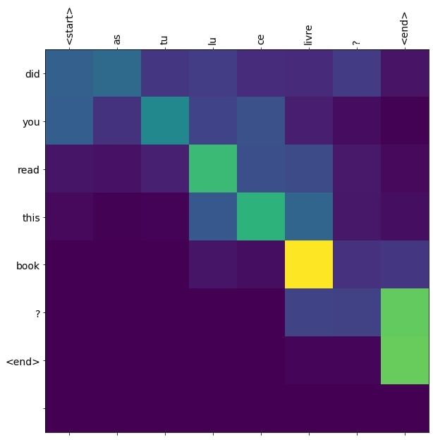 

The actual translation is "Have you read this book?"

translate(u"Comment as-tu été?")

# Output
Input: <start> comment as tu ete ? <end>
Predicted translation: how were you ? <end>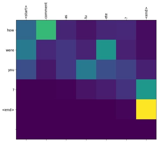 

The actual translation is "How have you been?"

As can be inferred, the predicted translations are in proximity to the actual translations.

Conclusion

This is the final part of my series on RNNs. In this tutorial, you’ve learned what the Attention Mechanism is all about. You’ve learned how it fares better than a general encoder-decoder sequence-to-sequence model. You’ve also trained a neural machine translation model to convert sentences from French to English. You can further tweak the model’s hyperparameters to measure how the model’s performing.

I hope you enjoyed reading this series!

Reference: TensorFlow Tutorial