Understanding Hough Transform With A Lane Detection Model

The hough transform technique is an amazing tool that can be used for locating shapes in images. It is often used to detect circles, ellipses, and lines to get the exact location or geometrical understanding of the image. This ability of the Hough transform to identify shapes makes it an ideal tool for detecting lane lines for a self-driving car.

Lane detection is one of the basic concepts when trying to understand how self-driving cars work. In this article, we will build a program that can identify lane lines in a picture or a video and learn how the Hough transform plays a huge role in achieving this task. Hough transform comes almost as the last step in detecting straight lines in the region of interest. Since it is also important to know how we get to that stage, be patient as we go through each step.

Table of Contents

1. Project Setup
2. Load & Display Image
3. Canny Edge Detection: Gray-Scaling, Noise Reduction, Canny Method
4. Isolating Region Of Interest (ROI)
5. Hough Transform Technique
6. Implementing Hough Transform
7. Detecting Lanes In Video
8. Final Thoughts

Project Setup

When humans are driving a car, we see the lanes with our eyes. But since a car cannot do that, we use computer vision to make it "see" the lane lines. We are going to use OpenCV to read and display the series of pixels in our image.

To get started,

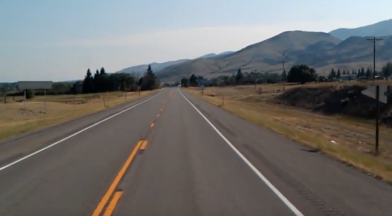
• Install this image and save it in a folder as a JPEG file.
• Open an IDE and create a python file in the same folder. Let's name it lanes.py
• Install openCV from the terminal with the command - pip install opencv-contrib-python

Load & Display The Image

The openCV library has a function called cv2.imread() which loads the image from our file and returns it as a multi-dimensional NumPy array.

import cv2
image = cv2.imread('lane.jpg')

The NumPy array represents the relative intensities of each pixel in the image.

We now have our image data in the form of an array. The next step is to render our image with a function called imshow() . This takes in two arguments - the first being the name of the window where our image is displayed and the second being the image we want to show.

import cv2

image = cv2.imread('lane.jpg')
cv2.imshow('result', image)
cv2.waitKey(0)

The waitKey() function allows us to display the image for a specified amount of milliseconds. The '0' here, says the function to show the image infinitely until we press anything on our keyboard.

Open the terminal and run the program with python lanes.py and you should see the image displayed on your screen.

Canny Edge Detection

In this section, we will discuss canny edge detection, a technique that we will use to write a program that will detect the edges in an image. Therefore we try to find the areas in an image where there is a sharp change in intensity and a sharp change in color.

It is important to keep in mind that an image can be read as a matrix (an array of pixels).  A pixel contains light intensities at some location in the image. Each pixel's intensity is denoted by numeric values arranged from 0 to 255. The 0 value indicates no intensity (black), and 255 indicates maximum intensity (white).  

Note: Gradient is a measure of change in brightness over a series of pixels. A strong gradient represents a drastic change, whereas a small gradient shows a shallow change.

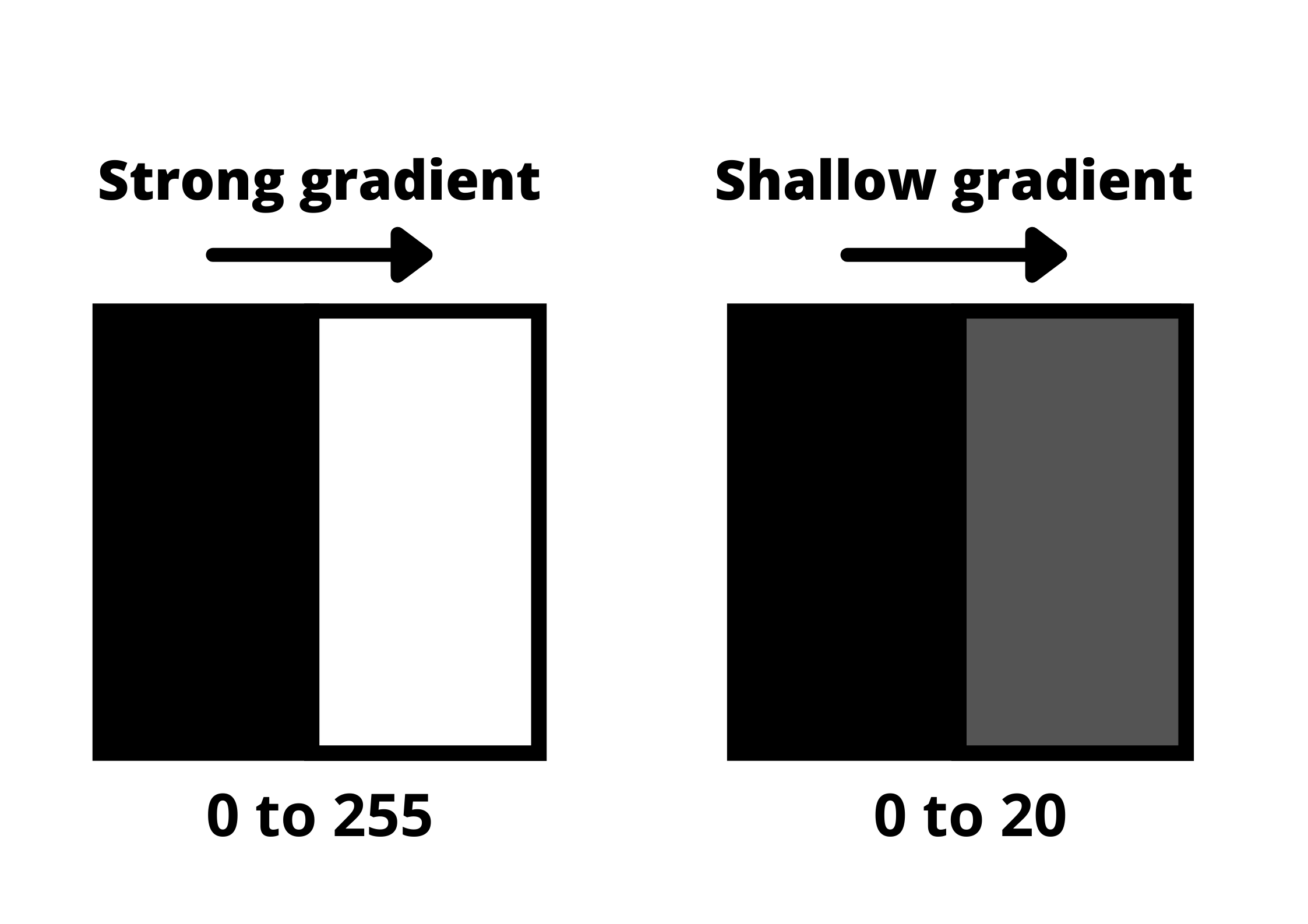
The strengthening of gradients helps us identify edges in our image. An edge is defined by the difference in intensity values in adjacent pixels. Whenever you see a sharp change in intensity or a rapid change in brightness, there is a corresponding bright pixel in the gradient image. By tracing these pixels, we obtain the edges.

Now, we are going to apply this intuition to detect edges on our image. There are three steps involved in this process.

Step-1: Gray-Scaling

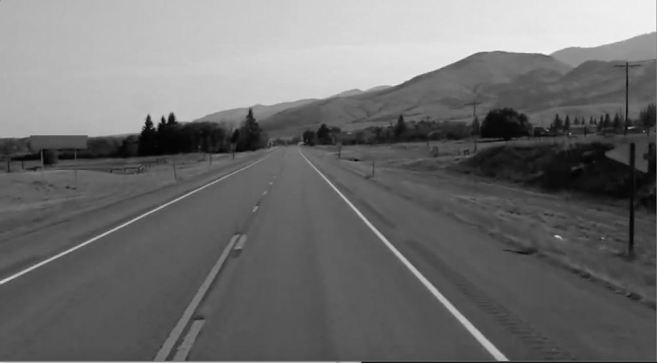
The reason for converting our image to grayscale is to process it easily. The gray-scale image has only a one-pixel intensity value (0 or 1) compared to a colored image which has more than three values. This will make the gray-scale image work in a single channel, which will be easier and faster for us to process rather than three channeled color pictures.

To implement this in code, we are going to make a copy of the image array created previously with the help of NumPy.

image = cv2.imread('lane.jpg')
lane_image = np.copy(image) #creating copy of the image

It is important to create a copy of the image variable rather than setting the new variable equal to the image. Doing this will ensure that the changes made in  lane_image do not affect image .

Now, we convert the image to grayscale with the help of cvtColor function from our openCV library.

gray = cv2.cvtColor(lane_image, cv2.COLOR_RGB2GRAY) #converting to gray-scale

The flag COLOR_RGB2GRAY is passed as a second argument and helps in the conversion of RGB color to a grayscale image.

To output this conversion, we need to pass gray in our resulting window.

import cv2
import numpy as np

image = cv2.imread('lane.jpg')
lane_image = np.copy(image)
gray = cv2.cvtColor(lane_image, cv2.COLOR_RGB2GRAY) 

cv2.imshow('result', gray) #to output gray-scale image
cv2.waitKey(0)

If we run this program, the resulting image should be as shown below.

Step-2: Reduce Noise & Smoothen

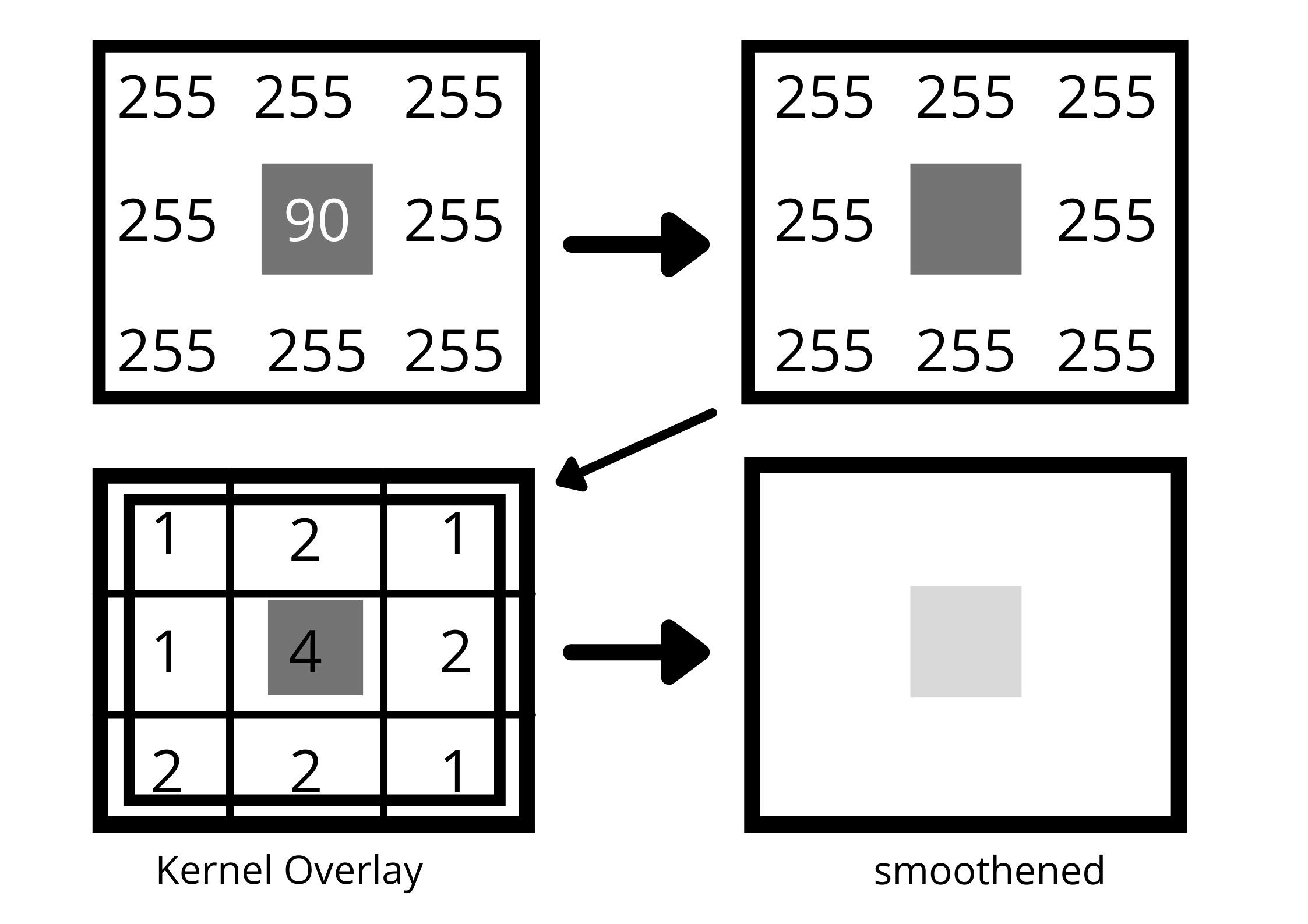
It is important to identify as many edges in the image as possible. But, we must also filter any image noise which can create false edges and ultimately affect edge detection. This reduction of noise and image smoothening will be done by a filter called Gaussian Blur.

Remember that an image is stored as a collection of discrete pixels. Each pixel in a gray-scale image is represented by a single number that describes the brightness of the pixel. To smoothen an image, we need to modify the value of a pixel with the average value of pixel intensities around it.

Averaging of pixels to reduce noise will be done with a kernel. This kernel window of normally distributed numbers is run across our entire image and sets each pixel value equal to the weighted average of its neighboring pixel, thus smoothening our image.

To represent this convolution in code, we apply cv2.GaussianBlur() function on our grayscale image.

blur = cv2.GaussianBlur(gray, (5, 5), 0)

Here, we are applying a 5 * 5 kernel window on our image. The size of the kernel depends on the situation but a 5*5 window is ideal for most cases. We pass the blur variable to imshow() to get the output. Therefore, the final code to obtain a Gaussian blur image looks like this:

import cv2
import numpy as np

image = cv2.imread('lane.jpg')
lane_image = np.copy(image)
gray = cv2.cvtColor(lane_image, cv2.COLOR_RGB2GRAY) 
blur = cv2.GaussianBlur(gray, (5, 5), 0)

cv2.imshow('result', blur) #to output gaussian image.
cv2.waitKey(0)

The resulting is a blurred image obtained by convolving a kernel of Gaussian values that have reduced noise.

Note: This is an optional step to understand gaussian blur. When we perform canny edge detection in the next step, it automatically performs this for us.

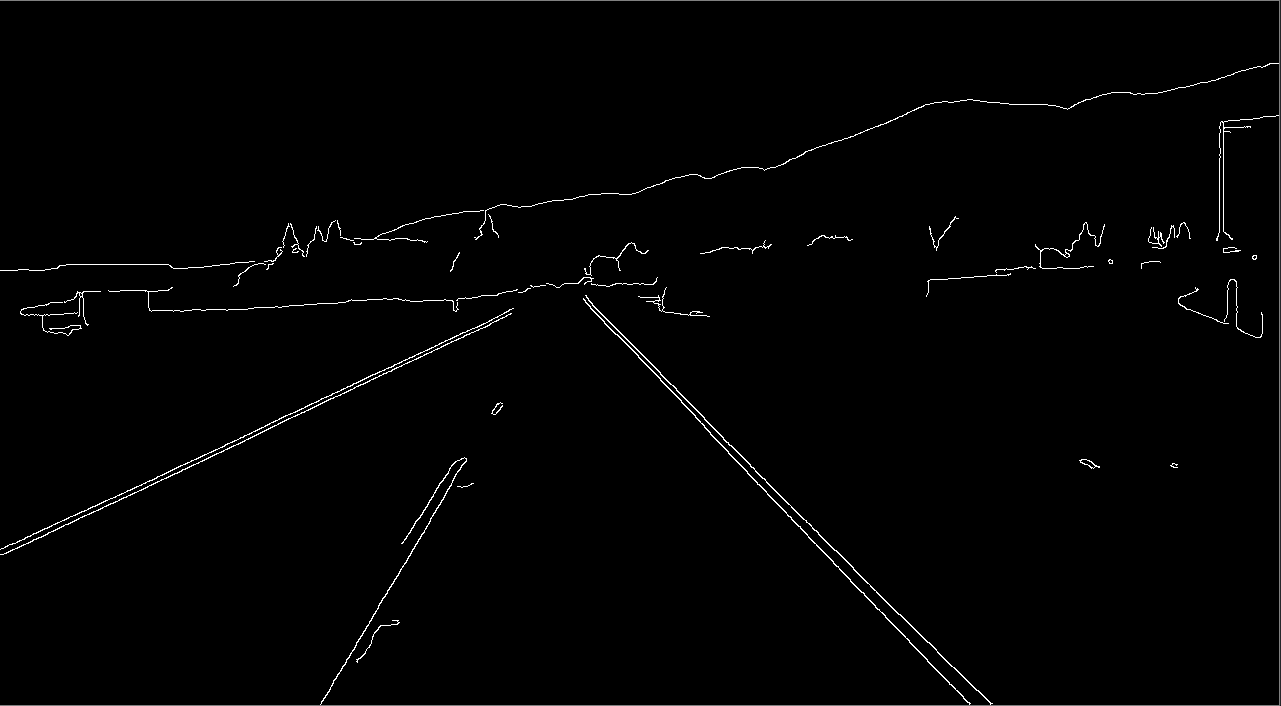
Step-3: Canny Method

To understand this concept, you must recall that an image can also be represented in a 2D coordinate space - X & Y.

X corresponds to the width (no. of columns) in the image and Y corresponds to the height (no. of rows) of an image. The product of both width and height gives us the total number of pixels in an image. This tells us that we can not only represent images as an array but also as a continuous function of X and Y i.e; f(x, y).

Since f(x, y) is a mathematical function, we can perform operations to determine rapid changes in the brightness of the pixels in an image. The canny method will give us a derivative of our function in both x and y directions. We can use this derivative to measure the change in intensities concerning adjacent pixels.

A small change in derivative corresponds to a small change in intensity and vice versa.

By computing the derivatives in all directions, we get the gradient of the image. Calling the cv2.Canny() function in our code performs all of these actions for us.

cv2.Canny(image, low_threshold, high_threshold)

This function will trace the strongest gradience as a series of white pixels. The two arguments low_threshold and high_threshold  allows us to isolate the adjacent pixels that follow the strongest gradience. If the gradient is larger than the upper threshold, then it is identified as an edge pixel. If it's below the lower threshold, it gets rejected. The gradient between the thresholds is accepted only when it is connected to a strong edge.

For our case, we're going to take a low-high threshold ratio of 1:3. This time we output the canny image instead of the blurred image.

canny = cv2.Canny(blur, 50, 150) #to obtain edges of the image
cv2.imshow('result', Canny)
cv2.waitKey(0)

The resulting image looks something like this:

Isolating Region Of Interest (ROI)

Before we teach our model to detect, we have to specify the region we are interested to detect the lane lines at.

In this case, let's take the region of interest as the right side of the road as shown in the figure.

Since we have a lot of variables and functions in our code, now would be a good time to wrap everything by defining a function.

import cv2
import numpy as np

def canny(image):
    gray = cv2.cvtColor(image, cv2.COLOR_RGB2GRAY)
    blur = cv2.GaussianBlur(gray,(5, 5), 0)
    canny = cv2.Canny(blur, 50, 150)
    return canny
    
image = cv2.imread('lane.jpg')
lane_image = np.copy(image)
canny = cv2.Canny(lane_image) 
cv2.imshow('result', canny)
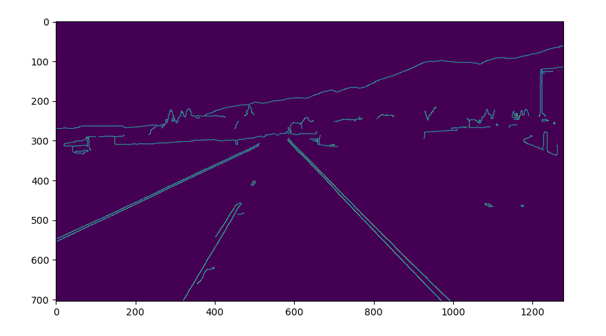
cv2.waitKey(0)

To clarify the exact position of our region of interest, we use matplotlib library to spot the coordinates and isolate that region.

import cv2
import numpy as np
import matplotlib.pyplot as plt

def canny(image):
    gray = cv2.cvtColor(image, cv2.COLOR_RGB2GRAY)
    blur = cv2.GaussianBlur(gray,(5, 5), 0)
    canny = cv2.Canny(blur, 50, 150)
    return canny
    
image = cv2.imread('lane.jpg')
lane_image = np.copy(image)
canny = cv2.Canny(lane_image) 
plt.imshow(canny)
plt.show()

Running this gives us an image with X and Y coordinates corresponding to our region of interest.

Now that we have the required measurements for our ROI, we are going to generate an image that will mask everything else. The image we get is a mask of the polygon with specified vertices from our original image.

def region_of_interest(image):
    height = image.shape[0]
    polygons = np.array([
    [(200, height), (1100, height), (550, 250)]
    ])
    mask = np.zeros_like(image)
    cv2.fillPoly(mask, polygons, 255)
    return mask
	
 ...
  
cv2.imshow('result', region_of_interest(canny)) #changing it to show ROI instead of canny image.

...

The code above is pretty self-explanatory. It returns the enclosed region of our field view which is triangular.

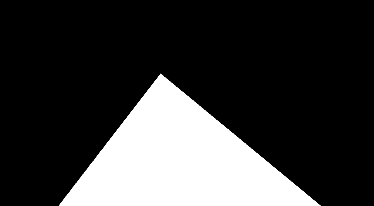
This image is important because it represents our region of interest with a strong gradient difference. The pixel intensity values in the triangular region are 255 and for the rest of the image, it is zero. Since this image has the same measurements as our original image, it can be used to easily extract the lines from our previously generated canny image.

we can implement this by utilizing cv2.bitwise_and() function from OpenCV, which computes the bitwise & of both images to only show the ROI traced by the polygonal contour of the mask. Refer to openCV documentation for more information on using bitwise_and .

def region_of_interest(image):
    height = image.shape[0]
    polygons = np.array([
    [(200, height), (1100, height), (550, 250)]
    ])
    mask = np.zeros_like(image)
    cv2.fillPoly(mask, polygons, 255)
	masked_image = cv2.bitwise_and(image, mask)
    return masked_image

...

cropped_image = region_of_interest(canny)
cv2.imshow('result', cropped_image)

...

You should expect an output that looks as follows -

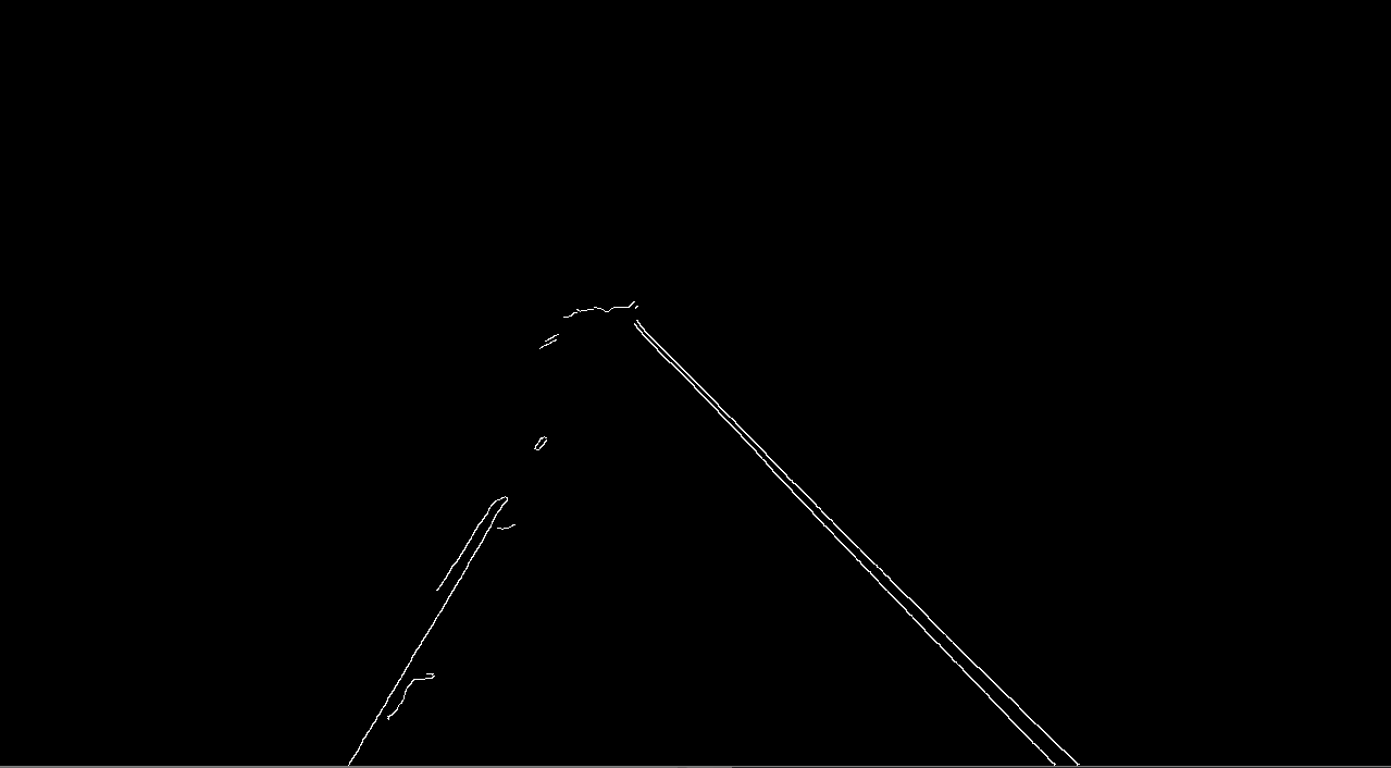
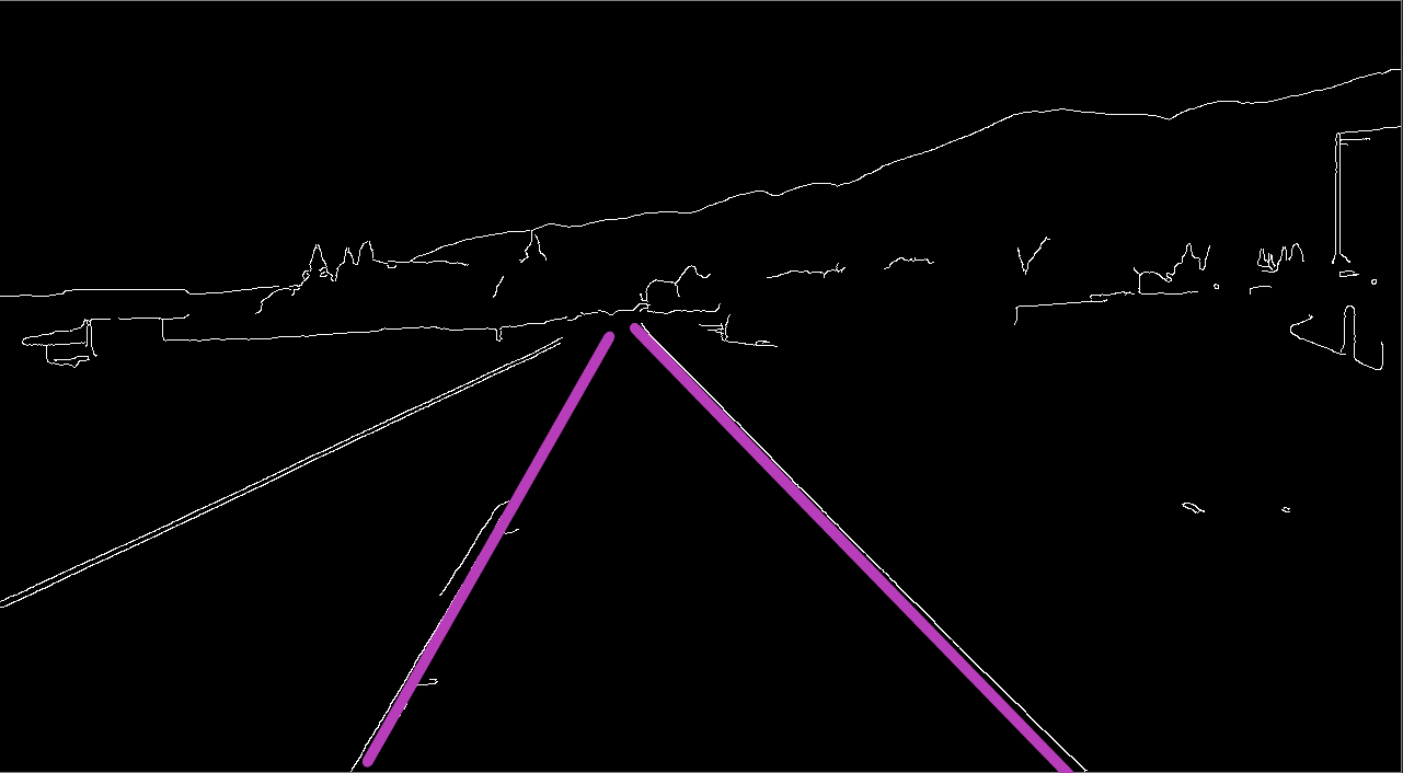
The final step in this process is to use hough transform to detect straight lines in our isolated region of interest.

Hough Transform Technique

The picture we have right now is just a series of pixels and we cannot find a geometrical representation directly to know the slope and intercepts.

Since images are never perfect, we cannot loop through the pixels to find the slope and intercept since it would be a very difficult task. This is where hough transform can be used. It helps us to figure out the prominent lines and connect the disjoint edge points in an image.

Let's understand this concept by comparing normal X-Y co-ordinate space and hough space (M-C space).

A point in an XY plane can have any number of lines passing through it. The same is true if we take a line in the same XY plane, many points are passing through that line.

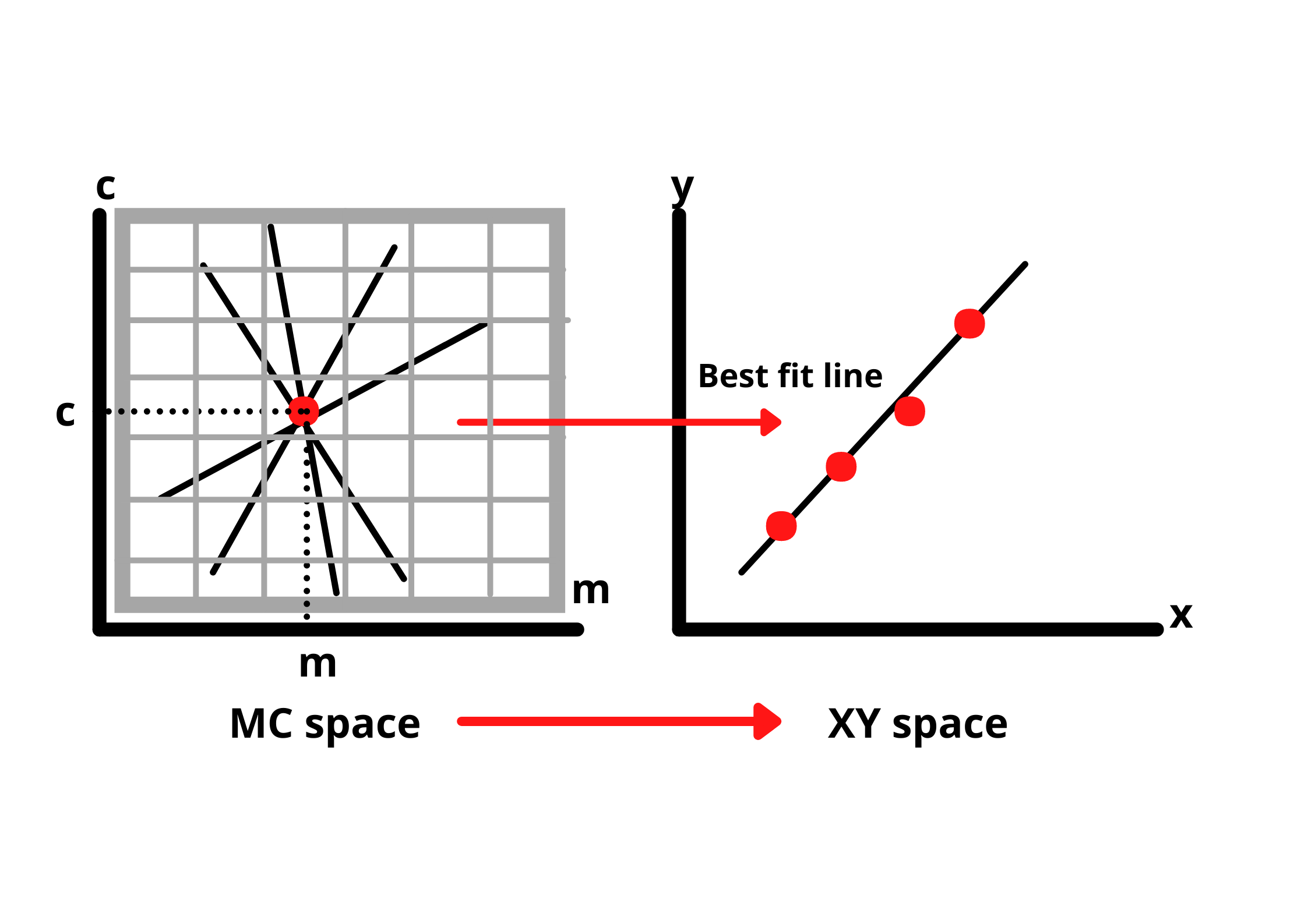
To identify the lines in our picture, we have to imagine each edge pixel as a point in a co-ordinate space and we are going to convert that point into a line in the hough space.

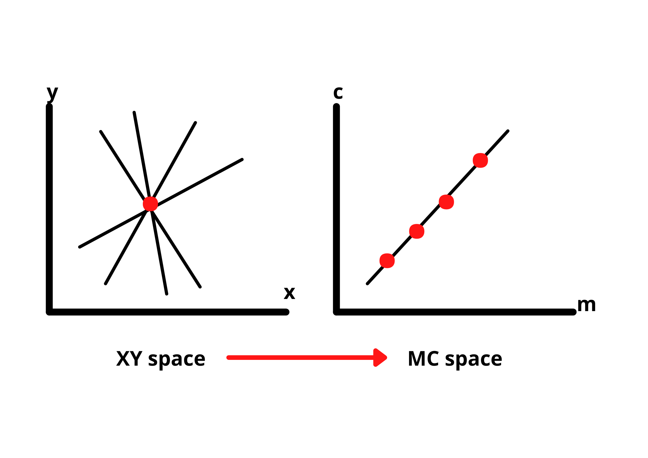
We need to find two or more lines representing their corresponding points(on XY-plane) that intersect in the hough space to detect the lines. This way we know that the two points belong to the same line.

The idea of finding possible lines from a series of points is how we can find the lines in our gradient image. But, the model also needs parameters of the lines to identify them.

To get these parameters, we first divide the hough space into a grid containing small squares as shown in the figure. The values of c and m corresponding to the square with the most number of intersections will be used to draw the best fit line.

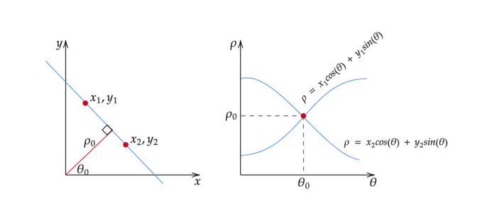
This approach works well with lines that have slopes. But, if we are dealing with a straight line, the slope will always be infinity and we cannot exactly work with that value. So, we make a small change in our approach.

Instead of representing our line equation as y = mx + c, we express it in the polar co-ordinate system i.e; ρ = Xcosθ + Ysinθ.

• ρ = perpendicular distance from the origin.
• θ = angle of inclination of the normal line from the x-axis.

By representing the line in polar coordinates, we get a sinusoidal curve in the hough space instead of straight lines. This curve is identified for all of the different values for ρ and θ of lines passed through our points. If we have more points, they create more curves in our hough space. Similar to the previous case, the values corresponding to the most intersecting curves, will be taken to create the best fit line.

Implementing Hough Transform

Since we finally have a technique to identify lines in our image, let's implement it in the code. Fortunately, openCV already has a function called cv2.HoughLinesP() that can be used to do this task for us.

lines = cv2.HoughLinesP(cropped_image, 2, np.pi/180, 100, np.array([]), minLineLength=40, maxLineGap=5)

The first argument is the cropped image that was generated earlier which is a gradient image of isolated lane lines. The second and third arguments specify the resolution of the hough accumulator array (the grid created to recognize most intersections). The fourth argument is the threshold value required to identify the minimum number of votes needed to detect a line.

Before displaying these lines in our real image, let's define few functions to represent them. We will define 3 functions to perfectly optimize and display the lane lines.

• display_lines: We define this function to mark the lines on a black image with similar measurements as the original image and then blend it into our color image.

def display_lines(image, lines):
    line_image = np.zeros_like(image)
    if lines is not None:
        for x1, y1, x2, y2 in lines:
            cv2.line(line_image, (x1, y1), (x2, y2), (255, 0, 0), 10)
    return line_image

We utilize cv2.addWeight() to combine the line image and the color image.

line_image = display_lines(lane_image, averaged_lines)

combo_image = cv2.addWeighted(lane_image, 0.8, line_image, 1, 1)

• make_coordinates: This will specify the coordinates for us to be able to mark the slope and y-intercept.

def make_coordinates(image, line_parameters):
    slope, intercept = line_parameters
    y1 = image.shape[0]
    y2 = int(y1*(3/5))
    x1 = int((y1 - intercept)/slope)
    x2 = int((y2 - intercept)/slope)
    return np.array([x1, y1, x2, y2])

• average_slope_intercept: we first declare two empty lists - left_fit and right_fit which will contain the coordinates of the average lines on the left and coordinates of the lines on the right respectively.

def average_slope_intercept(image, lines):
    left_fit = []
    right_fit = []
    for line in lines:
        x1, y1, x2, y2 = line.reshape(4)
        parameters = np.polyfit((x1, x2), (y1, y2), 1)
        slope = parameters[0]
        intercept = parameters[1]
        if slope < 0:
            left_fit.append((slope, intercept))
        else:
            right_fit.append((slope, intercept))
    left_fit_average = np.average(left_fit, axis=0)
    right_fit_average = np.average(right_fit, axis=0)
    left_line = make_coordinates(image, left_fit_average)
    right_line = make_coordinates(image, right_fit_average)
    return np.array([left_line, right_line])

The np.polyfit() will give us the parameters of straight lines that will fit our points and returns a vector of coefficients that describes the slope and y-intercept.

Finally, we show the combo_image() where our lane lines are perfectly detected.

cv2.imshow('result', combo_image)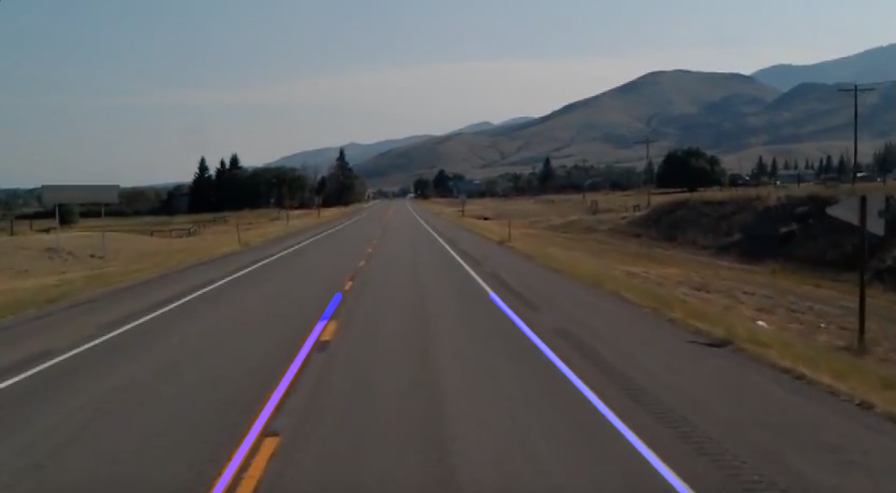

Detecting Lanes In Video

The same process is followed to detect lanes in a video. This is made easy by the VideoCapture object by OpenCV. This object lets you read frame by frame and perform the operations that you need.

Once you download this video, move it to the project folder where you're currently working.

We set up a video capture object for our video and apply the algorithm we already implemented to detect lines in the video instead of a static image.

cap = cv2.VideoCapture('test2.mp4')
while(cap.isOpened()):
    _, frame = cap.read()
    canny_image = canny(frame)
    cropped_image = region_of_interest(canny_image)
    lines = cv2.HoughLinesP(cropped_image, 2, np.pi/180, 100, np.array([]), minLineLength=40, maxLineGap=5)
    averaged_lines = average_slope_intercept(frame, lines)
    line_image = display_lines(frame, averaged_lines)
    combo_image = cv2.addWeighted(frame, 0.8, line_image, 1, 1)
    cv2.imshow('result',combo_image)
    if cv2.waitKey(1) == ord('q'):
        break
cap.release()
cv2.destroyAllWindows()

Note: while trying to implement the function above, it is a good idea to comment off the code related to the static images and keep it for later.

#image = cv2.imread('lane.jpg')
#lane_image = np.copy(image)

#canny_image = canny(lane_image)
#cropped_image = region_of_interest(canny_image)
#lines = cv2.HoughLinesP(cropped_image, 2, np.pi/180, 100, np.array([]), minLineLength=40, maxLineGap=5)
#averaged_lines = average_slope_intercept(lane_image, lines)
#line_image = display_lines(lane_image, averaged_lines)

#combo_image = cv2.addWeighted(lane_image, 0.8, line_image, 1, 1)

#cv2.imshow('result',combo_image)
#cv2.waitKey(0)

If everything runs well, you will see the same lane lines in action, in your video.

This was a lot of explanation and it is common to get confused at some point. So, this is how your entire code on lanes.py should look like when you're done.

import cv2
import numpy as np

def make_coordinates(image, line_parameters):
    slope, intercept = line_parameters
    y1 = image.shape[0]
    y2 = int(y1*(3/5))
    x1 = int((y1 - intercept)/slope)
    x2 = int((y2 - intercept)/slope)
    return np.array([x1, y1, x2, y2])

def average_slope_intercept(image, lines):
    left_fit = []
    right_fit = []
    for line in lines:
        x1, y1, x2, y2 = line.reshape(4)
        parameters = np.polyfit((x1, x2), (y1, y2), 1)
        slope = parameters[0]
        intercept = parameters[1]
        if slope < 0:
            left_fit.append((slope, intercept))
        else:
            right_fit.append((slope, intercept))
    left_fit_average = np.average(left_fit, axis=0)
    right_fit_average = np.average(right_fit, axis=0)
    left_line = make_coordinates(image, left_fit_average)
    right_line = make_coordinates(image, right_fit_average)
    return np.array([left_line, right_line])

def canny(image):
    gray = cv2.cvtColor(image, cv2.COLOR_RGB2GRAY)
    blur = cv2.GaussianBlur(gray,(5, 5), 0)
    canny = cv2.Canny(blur, 50, 150)
    return canny

def display_lines(image, lines):
    line_image = np.zeros_like(image)
    if lines is not None:
        for x1, y1, x2, y2 in lines:
            cv2.line(line_image, (x1, y1), (x2, y2), (255, 0, 0), 10)
    return line_image

def region_of_interest(image):
    height = image.shape[0]
    polygons = np.array([
    [(200, height), (1100, height), (550, 250)]
    ])
    mask = np.zeros_like(image)
    cv2.fillPoly(mask, polygons, 255)
    masked_image = cv2.bitwise_and(image, mask)
    return masked_image

#image = cv2.imread('lane.jpg')
#lane_image = np.copy(image)

#canny_image = canny(lane_image)
#cropped_image = region_of_interest(canny_image)
#lines = cv2.HoughLinesP(cropped_image, 2, np.pi/180, 100, np.array([]), minLineLength=40, maxLineGap=5)
#averaged_lines = average_slope_intercept(lane_image, lines)
#line_image = display_lines(lane_image, averaged_lines)

#combo_image = cv2.addWeighted(lane_image, 0.8, line_image, 1, 1)

#cv2.imshow('result',combo_image)
#cv2.waitKey(0)

cap = cv2.VideoCapture('test2.mp4')
while(cap.isOpened()):
    _, frame = cap.read()
    canny_image = canny(frame)
    cropped_image = region_of_interest(canny_image)
    lines = cv2.HoughLinesP(cropped_image, 2, np.pi/180, 100, np.array([]), minLineLength=40, maxLineGap=5)
    averaged_lines = average_slope_intercept(frame, lines)
    line_image = display_lines(frame, averaged_lines)
    combo_image = cv2.addWeighted(frame, 0.8, line_image, 1, 1)
    cv2.imshow('result',combo_image)
    if cv2.waitKey(1) == ord('q'):
        break
cap.release()
cv2.destroyAllWindows()

Final Thoughts

This is a simple example of a lane detection model. You can take this project further to make the algorithm adapt to real-time video data and detect the lane lines as the car moves.

Congratulations on making it this far! Hopefully, you found this tutorial helpful and explore more areas related to this concept.