In another post, we covered the nuts and bolts of Stochastic Gradient Descent and how to address problems like getting stuck in a local minima or a saddle point. In this post, we take a look at another problem that plagues training of neural networks, pathological curvature.
While local minima and saddle points can stall our training, pathological curvature can slow down training to an extent that the machine learning practitioner might think that search has converged to a sub-optimal minma. Let us understand in depth what pathological curvature is.
Pathological Curvature
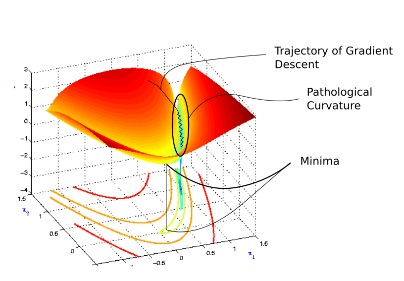
Consider the following loss contour.
**Pathological Curvature**
You see, we start off randomly before getting into the ravine-like region marked by blue color. The colors actually represent how high the value the loss function is at a particular point, with reds representing highest values and blues representing the lowest values.
We want to get down to the minima, but for that we have move through the ravine. This region is what is called pathological curvature. To understand why it's called pathological , let us delve deeper. This is how pathological curvature, zoomed up, looks like..
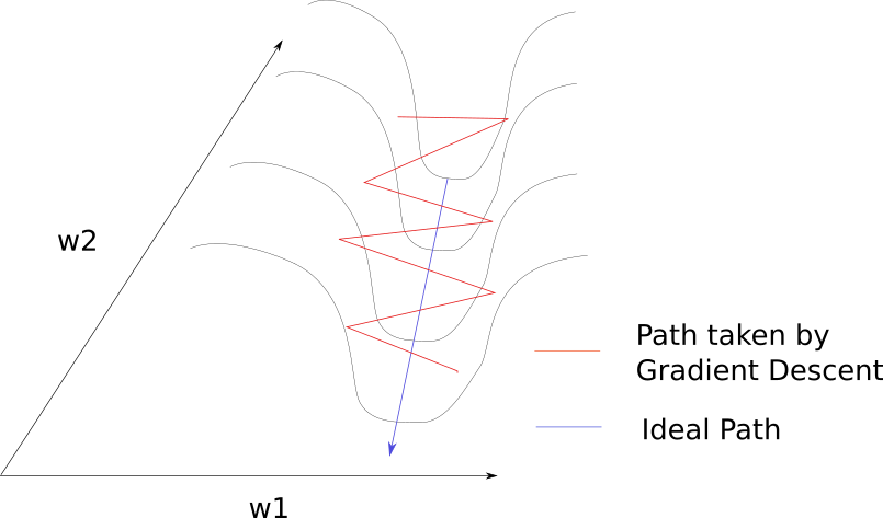
**Pathological Curvature**
It's not very hard to get hang of what is going on in here. Gradient descent is bouncing along the ridges of the ravine, and moving a lot slower towards the minima. This is because the surface at the ridge curves much more steeply in the direction of w1.
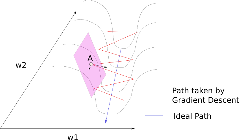
Consider a point A, on the surface of the ridge. We see, the gradient at the point can be decomposed into two components, one along direction w1 and other along w2. The component of the gradient in direction of w1 is much larger because of the curvature of the loss function, and hence the direction of the gradient is much more towards w1, and not towards w2 (along which the minima lies).
Normally, we could use a slow learning rate to deal with this bouncing between the ridges problem as we covered in the last post on gradient descent. However, this spells trouble.
It makes sense to slow down when were are nearing a minima, and we want to converge into it. But consider the point where gradient descent enters the region of pathological curvature, and the sheer distance to go until the minima. If we use a slower learning rate, it might take so too much time to get to the minima. In fact, one paper reports that learning rates small enough to prevent bouncing around the ridges might lead the practitioner to believe that the loss isn't improving at all, and abandon training all together.
And if the only directions of significant decrease in f are ones of low curvature, the optimization may become too slow to be practical and even appear to halt altogether, creating the false impression of a local minimum
Probably we want something that can get us slowly into the flat region at the bottom of pathological curvature first, and then accelerate in the direction of minima. Second derivatives can help us do that.
Newton's Method
Gradient descent is a First Order Optimization Method. It only takes the first order derivatives of the loss function into account and not the higher ones. What this basically means it has no clue about the curvature of the loss function. It can tell whether the loss is declining and how fast, but cannot differentiate between whether the curve is a plane, curving upwards or curving downwards.
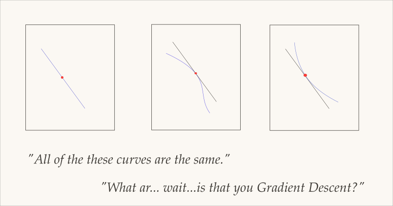
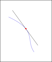
This happens because gradient descent only cares about the gradient, which is the same at the red point for all of the three curves above. The solution? Take into account double derivative, or the rate of how quickly the gradient is changing.
A very popular technique that can use second order derivatives to fix our issue is called the Newton's Method. For sake of not straying away from the topic of post, I won't delve much into the math of Newton's method. What I'll do instead is try to build an intuition of what Newton's Method does.
Newton's method can give us an ideal step size to move in the direction of the gradient. Since we now have information about the curvature of our loss surface, the step size can be accordingly chosen to not overshoot the floor of the region with pathological curvature.
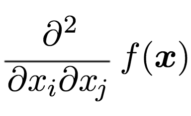
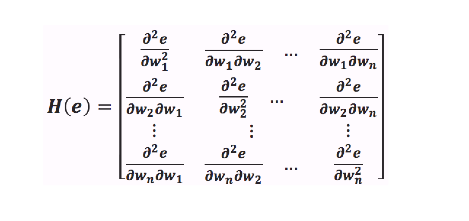
Newton's Method does it by computing the Hessian Matrix, which is a matrix of the double derivatives of the loss function with respect of all combinations of the weights. What I mean by saying a combination of the weights, is something like this.
A Hessian Matrix then accumulates all these gradients in one large big matrix.
The Hessian gives us an estimate of the curvature of loss surface at a point. A loss surface can have a positive curvature which means the surface, which means a surface is rapidly getting less steeper as we move. If we have a negative curvature, it means that the surface is getting more steeper as we move.
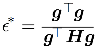
Notice, if this step is negative, it means we can use a arbitrary step. In other words, we can just switch back to our original algorithm. This corresponds to the following case where the gradient is getting more steeper.
However if the gradient is getting less steeper, we might be heading towards a region at the bottom of pathological curvature. Here, Newton's algorithm gives us a revised learning step, which is, as you can see is inversely proportional to the curvature, or how quickly the surface is getting less steeper.
If the surface is getting less steeper, then the learning step is decreased.
So why don't we use Newton's algorithm more often?
You see that Hessian Matrix in the formula? That hessian requires you to compute gradients of the loss function with respect to every combination of weights. If you know your combinations, that value is of the order of the square of the number of weights present in the neural network.
For modern day architectures, the number of parameters may be in billions, and calculating a billion squared gradients makes it computationally intractable for us to use higher order optimization methods.
However, here's an idea. Second order optimization is about incorporating the information about how is the gradient changing itself. Though we cannot precisely compute this information, we can chose to follow heuristics that guide our search for optima based upon the past behavior of gradient.
Momentum
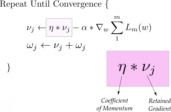
A very popular technique that is used along with SGD is called Momentum. Instead of using only the gradient of the current step to guide the search, momentum also accumulates the gradient of the past steps to determine the direction to go. The equations of gradient descent are revised as follows.

The first equations has two parts. The first term is the gradient that is retained from previous iterations. This retained gradient is multiplied by a value called "Coefficient of Momentum" which is the percentage of the gradient retained every iteration.
If we set the initial value for v to 0 and chose our coefficient as 0.9, the subsequent update equations would look like.

We see that the previous gradients are also included in subsequent updates, but the weightage of the most recent previous gradients is more than the less recent ones. (For the mathematically inclined, we are taking an exponential average of the gradient steps)
How does this help our case. Consider the image,and notice that most of the gradient updates are in a zig-zag direction. Also notice that each gradient update has been resolved into components along w1 and w2 directions. If we will individually sum these vectors up, their components along the direction w1 cancel out, while the component along the w2 direction is reinforced.
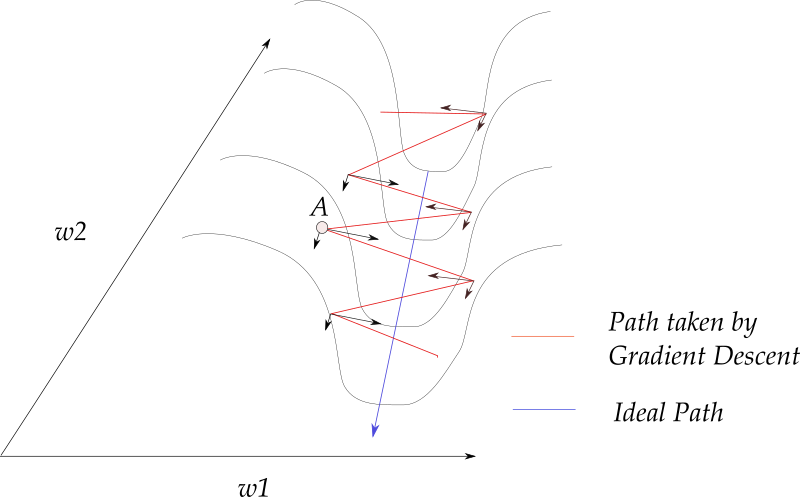
For an update, this adds to the component along w2, while zeroing out the component in w1 direction. This helps us move more quickly towards the minima. For this reason, momentum is also referred to as a technique which dampens oscillations in our search.
It also builds speed, and quickens convergence, but you may want to use simulated annealing in case you overshoot the minima.
In practice, the coefficient of momentum is initialized at 0.5, and gradually annealed to 0.9 over multiple epochs.
RMSProp
RMSprop, or Root Mean Square Propogation has an interesting history. It was devised by the legendary Geoffrey Hinton, while suggesting a random idea during a Coursera class.
RMSProp also tries to dampen the oscillations, but in a different way than momentum. RMS prop also takes away the need to adjust learning rate, and does it automatically. More so, RMSProp choses a different learning rate for each parameter.
In RMS prop, each update is done according to the equations described below. This update is done separately for each parameter.

So, let's break down what is happening here.
In the first equation, we compute an exponential average of the square of the gradient. Since we do it separately for each parameter, gradient Gt here corresponds to the projection, or component of the gradient along the direction represented by the parameter we are updating.
To do that, we multiply the exponential average computed till the last update with a hyperparameter, represented by the greek symbol nu. We then multiply the square of the current gradient with (1 - nu). We then add them together to get the exponential average till the current time step.
The reason why we use exponential average is because as we saw, in the momentum example, it helps us weigh the more recent gradient updates more than the less recent ones. In fact, the name "exponential" comes from the fact that the weightage of previous terms falls exponentially (the most recent term is weighted as p, the next one as squared of p, then cube of p, and so on.)
Notice our diagram denoting pathological curvature, the components of the gradients along w1 are much larger than the ones along w2. Since we are squaring and adding them, they don't cancel out, and the exponential average is large for w2 updates.
Then in the second equation, we decided our step size. We move in the direction of the gradient, but our step size is affected by the exponential average. We chose an initial learning rate eta, and then divide it by the average. In our case, since the average of w1 is much much larger than w2, the learning step for w1 is much lesser than that of w2. Hence, this will help us avoid bouncing between the ridges, and move towards the minima.
The third equation is just the update step. The hyperparameter p is generally chosen to be 0.9, but you might have to tune it. The epsilon is equation 2, is to ensure that we do not end up dividing by zero, and is generally chosen to be 1e-10.
It's also to be noted that RMSProp implicitly performs simulated annealing. Suppose if we are heading towards the minima, and we want to slow down so as to not to overshoot the minima. RMSProp automatically will decrease the size of the gradient steps towards minima when the steps are too large (Large steps make us prone to overshooting)
Adam
So far, we've seen RMSProp and Momentum take contrasting approaches. While momentum accelerates our search in direction of minima, RMSProp impedes our search in direction of oscillations.
Adam or Adaptive Moment Optimization algorithms combines the heuristics of both Momentum and RMSProp. Here are the update equations.

Here, we compute the exponential average of the gradient as well as the squares of the gradient for each parameters (Eq 1, and Eq 2). To decide our learning step, we multiply our learning rate by average of the gradient (as was the case with momentum) and divide it by the root mean square of the exponential average of square of gradients (as was the case with momentum) in equation 3. Then, we add the update.
The hyperparameter beta1 is generally kept around 0.9 while beta_2 is kept at 0.99. Epsilon is chosen to be 1e-10 generally.
Conclusion
In this post, we have seen 3 methods to build upon gradient descent to combat the problem of pathological curvature, and speed up search at the same time. These methods are often called "Adaptive Methods" since the learning step is adapted according to the topology of the contour.
Out of the above three, you may find momentum to be the most prevalent, despite Adam looking the most promising on paper. Empirical results have shown the all these algorithms can converge to different optimal local minima given the same loss. However, SGD with momentum seems to find more flatter minima than Adam, while adaptive methods tend to converge quickly towards sharper minima. Flatter minima generalize better than sharper ones.
Despite the fact that adaptive methods help us tame the unruly contours of a loss function of a deep net's loss function, they are not enough, especially with networks becoming deeper and deeper everyday. Along with choosing better optimization methods, considerable research is being put in coming up with architectures that produce smoother loss functions to start with. Batch Normalization and Residual Connections are a part of that effort, and we'll try to do a detailed blog post on them very shortly. But that's it for this post. Feel free to ask questions in the comments.