Image Credits: O'Reilly Media
Deep Learning, to a large extent, is really about solving massive nasty optimization problems. A Neural Network is merely a very complicated function, consisting of millions of parameters, that represents a mathematical solution to a problem. Consider the task of image classification. AlexNet is a mathematical function that takes an array representing RGB values of an image, and produces the output as a bunch of class scores.
By training neural networks, we essentially mean we are minimising a loss function. The value of this loss function gives us a measure how far from perfect is the performance of our network on a given dataset.
The Loss Function
Let us, for sake of simplicity, let us assume our network has only two parameters. In practice, this number would be around a billion, but we'll still stick to the two parameter example throughout the post so as not drive ourselves nuts while trying to visualise things. Now, the countour of a very nice loss function may look like this.

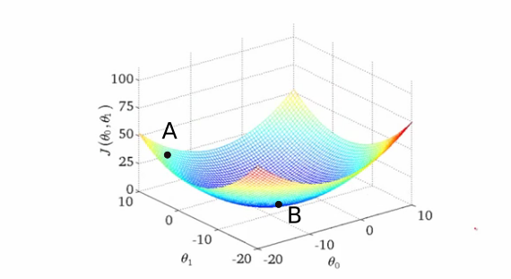
Contour of a Loss Function
Why do I say a very nice loss function? Because a loss function having a contour like above is like Santa, it doesn't exist. However, it still serves as a decent pedagogical tool to get some of the most important ideas about gradient descent across the board. So, let's get to it!
The x and y axes represent the values of the two weights. The z axis represents the value of the loss function for a particular value of two weights. Our goal is to find the particular value of weight for which the loss is minimum. Such a point is called a minima for the loss function.
You have randomly initialized weights in the beginning, so your neural network is probably behaving like a drunk version of yourself, classifying images of cats as humans. Such a situation correspond to point A on the contour, where the network is performing badly and consequently the loss is high.
We need to find a way to somehow navigate to the bottom of the "valley" to point B, where the loss function has a minima? So how do we do that?
Gradient Descent
Gradient Descent
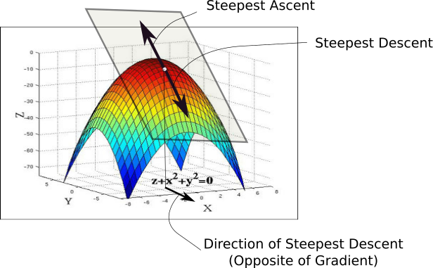
When we initialize our weights, we are at point A in the loss landscape. The first thing we do is to check, out of all possible directions in the x-y plane, moving along which direction brings about the steepest decline in the value of the loss function. This is the direction we have to move in. This direction is given by the direction exactly opposite to the direction of the gradient. The gradient, the higher dimensional cousin of derivative, gives us the direction with the steepest ascent.
To wrap your head around it, consider the following figure. At any point of our curve, we can define a plane that is tangential to the point. In higher dimensions, we can always define a hyperplane, but let's stick to 3-D for now. Then, we can have infinite directions on this plane. Out of them, precisely one direction will give us the direction in which the function has the steepest ascent. This direction is given by the gradient. The direction opposite to it is the direction of steepest descent. This is how the algorithm gets it's name. We perform descent along the direction of the gradient, hence, it's called Gradient Descent.
Now, once we have the direction we want to move in, we must decide the size of the step we must take. The the size of this step is called the learning rate. We must chose it carefully to ensure we can get down to the minima.
If we go too fast, we might overshoot the minima, and keep bouncing along the ridges of the "valley" without ever reaching the minima. Go too slow, and the training might turn out to be too long to be feasible at all. Even if that's not the case, very slow learning rates make the algorithm more prone to get stuck in a minima, something we'll cover later in this post.
Once we have our gradient and the learning rate, we take a step, and recompute the gradient at whatever position we end up at, and repeat the process.
While the direction of the gradient tells us which direction has the steepest ascent, it's magnitude tells us how steep the steepest ascent/descent is. So, at the minima, where the contour is almost flat, you would expect the gradient to be almost zero. In fact, it's precisely zero for the point of minima.

Gradient Descent in Action

Using too large a learning rate
In practice, we might never exactly reach the minima, but we keep oscillating in a flat region in close vicinity of the minima. As we oscillate our this region, the loss is almost the minimum we can achieve, and doesn't change much as we just keep bouncing around the actual minimum. Often, we stop our iterations when the loss values haven't improved in a pre-decided number, say, 10, or 20 iterations. When such a thing happens, we say our training has converged, or convergence has taken place.
A Common Mistake
Let me digress for a moment. If you google for visualizations of gradient descent, you'll probably see a trajectory that starts from a point and heads to a minima, just like the animation presented above. However, this gives you a very inaccurate picture of what gradient descent really is. The trajectory we take is entire confined to the x-y plane, the plane containing the weights.
As depicted in the above animation, gradient descent doesn't involve moving in z direction at all. This is because only the weights are the free parameters, described by the x and y directions. The actual trajectory that we take is defined in the x-y plane as follows.

Real Gradient Descent Trajectory
Each point in the x-y plane represents a unique combination of weights, and we want have a sets of weights described by the minima.
Basic Equations
The basic equation that describes the update rule of gradient descent is.

This update is performed during every iteration. Here, w is the weights vector, which lies in the x-y plane. From this vector, we subtract the gradient of the loss function with respect to the weights multiplied by alpha, the learning rate. The gradient is a vector which gives us the direction in which loss function has the steepest ascent. The direction of steepest descent is the direction exactly opposite to the gradient, and that is why we are subtracting the gradient vector from the weights vector.
If imagining vectors is a bit hard for you, almost the same update rule is applied to every weight of the network simultaneously. The only change is that since we are performing the update individually for each weight now, the gradient in the above equation is replaced the the projection of the gradient vector along the direction represented by the particular weight.

This update is simultaneously done for all the weights.
Before subtracting we multiply the gradient vector by the learning rate. This represents the step that we talked about earlier. Realise that even if we keep the learning rate constant, the size of step can change owing to changes in magnitude of the gradient, ot the steepness of the loss contour. As we approach a minima, the gradient approaches zero and we take smaller and smaller steps towards the minima.
In theory, this is good, since we want the algorithm to take smaller steps when it approaches a minima. Having a step size too large may cause it to overshoot a minima and bounce between the ridges of the minima.
A widely used technique in gradient descent is to have a variable learning rate, rather than a fixed one. Initially, we can afford a large learning rate. But later on, we want to slow down as we approach a minima. An approach that implements this strategy is called Simulated annealing, or decaying learning rate. In this, the learning rate is decayed every fixed number of iterations.
Challenges with Gradient Descent #1: Local Minima
Okay, so far, the tale of Gradient Descent seems to be a really happy one. Well. Let me spoil that for you. Remember when I said our loss function is very nice, and such loss functions don't really exists? They don't.
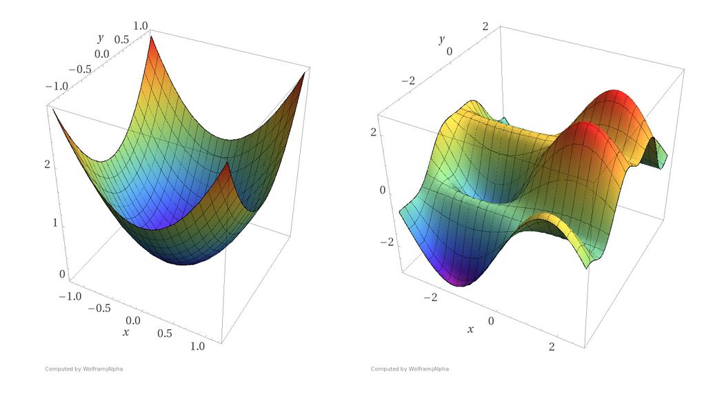
First, neural networks are complicated functions, with lots of non-linear transformations thrown in our hypothesis function. The resultant loss function doesn't look a nice bowl, with only one minima we can converge to. In fact, such nice santa-like loss functions are called convex functions (functions for which are always curving upwards) , and the loss functions for deep nets are hardly convex. In fact, they may look like this.
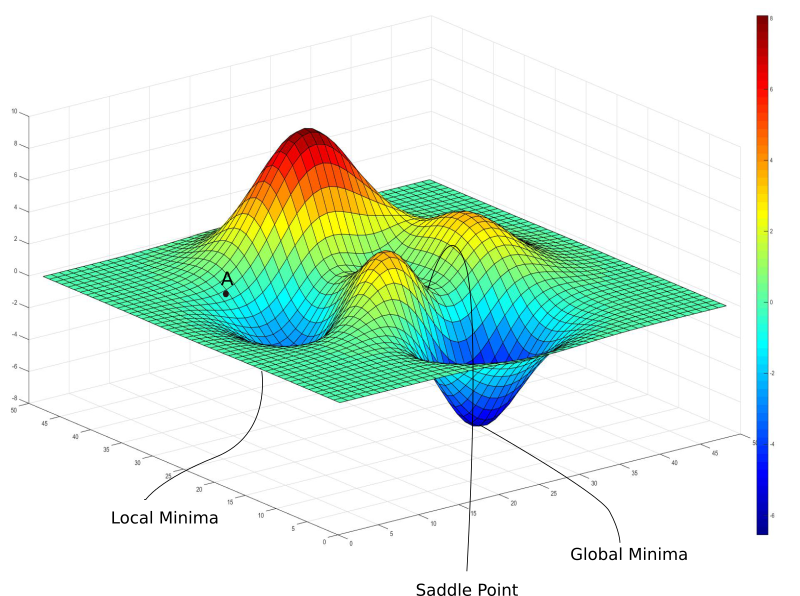
In the above image, there exists a local minima where the gradient is zero. However, we know that they are not the lowest loss we can achieve, which is the point corresponding to the global minima. Now, if you initialze your weights at point A, then you're gonna converge to the local minima, and there's no way gradient descent will get you out of there, once you converge to the local minima.
Gradient descent is driven by the gradient, which will be zero at the base of any minima. Local minimum are called so since the value of the loss function is minimum at that point in a local region. Whereas, a global minima is called so since the value of the loss function is minimum there, globally across the entire domain the loss function.
Only to make things worse, the loss contours even may be more complicated, given the fact that 3-d contours like the one we are considering never actually happen in practice. In practice, our neural network may have about, give or take, 1 billion weights, given us a roughly (1 billion + 1) dimensional function. I don't even know the number of zeros in that figure.
In fact, it's even hard to visualize what such a high dimensional function. However, given the sheer talent in the field of deep learning these days, people have come up with ways to visualize, the contours of loss functions in 3-D. A recent paper pioneers a technique called Filter Normalization, explaining which is beyond the scope of this post. However, it does give to us a view of the underlying complexities of loss functions we deal with. For example, the following contour is a constructed 3-D representation for loss contour of a VGG-56 deep network's loss function on the CIFAR-10 dataset.
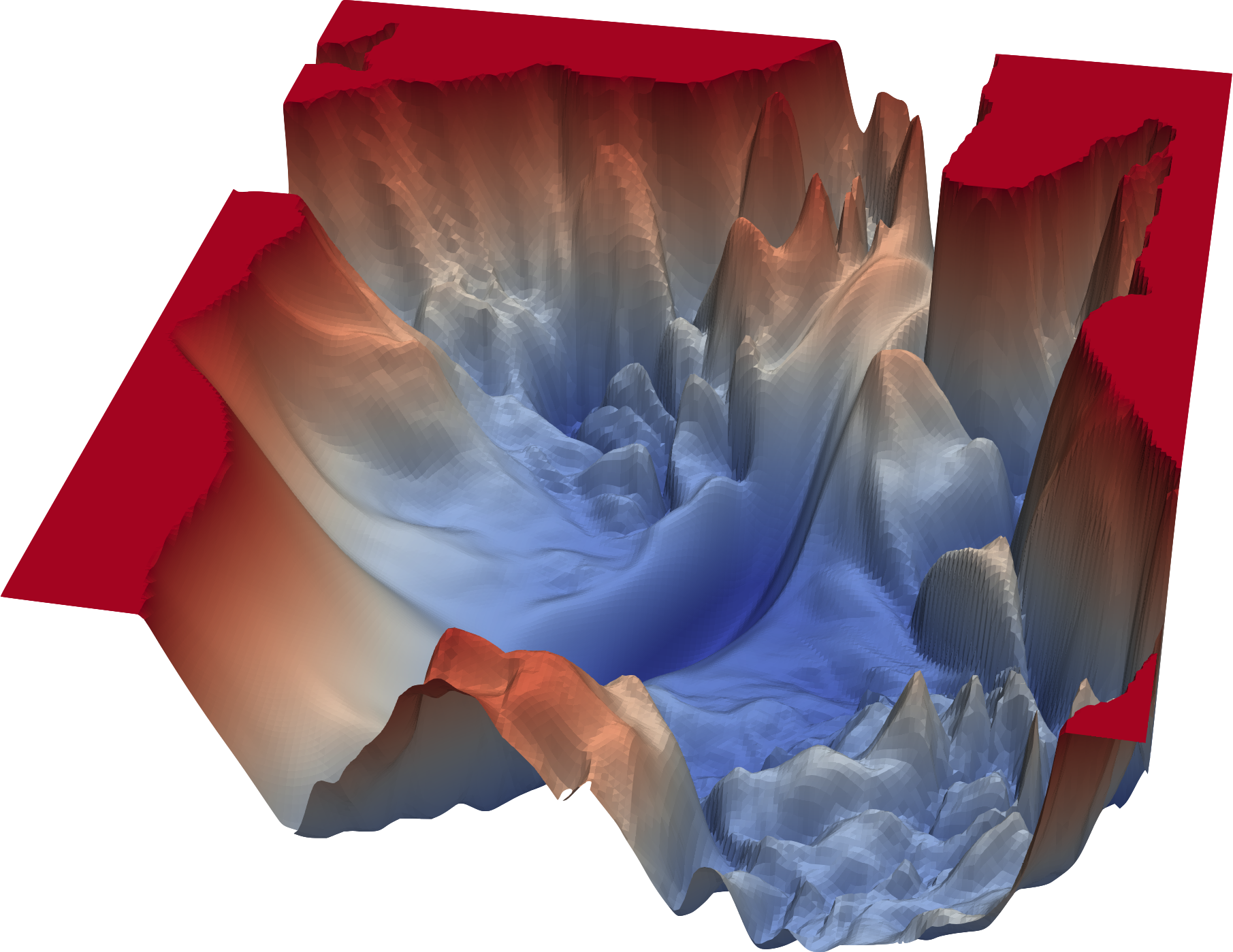
A Complicated Loss Landscape Image Credits: https://www.cs.umd.edu/~tomg/projects/landscapes/
As you can see, the loss landscape is ridden with local minimum.
Challenges with Gradient Descent #2: Saddle Points
The basic lesson we took away regarding the limitation of gradient descent was that once it arrived at a region with gradient zero, it was almost impossible for it to escape it regardless of the quality of the minima. Another sort of problem we face is that of saddle points, which look like this.
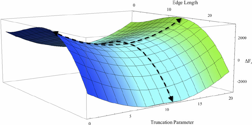
A Saddle Point
You can also see a saddle point in the earlier pic where two "mountains" meet.
A saddle point gets it's name from the saddle of a horse with which it resembles. While it's a minima in one direction (x), it's a local maxima in another direction, and if the contour is flatter towards the x direction, GD would keep oscillating to and fro in the y - direction, and give us the illusion that we have converged to a minima.
Randomness to the rescue!
So, how do we go about escaping local minima and saddle points, while trying to converge to a global minima. The answer is randomness.
Till now we were doing gradient descent with the loss function that had been created by summing loss over all possible examples of the training set. If we get into a local minima or saddle point, we are stuck. A way to help GD escape these is to use what is called Stochastic Gradient Descent.
In stochastic gradient descent, instead of taking a step by computing the gradient of the loss function creating by summing all the loss functions, we take a step by computing the gradient of the loss of only one randomly sampled (without replacement) example. In contrast to Stochastic Gradient Descent, where each example is stochastically chosen, our earlier approach processed all examples in one single batch, and therefore, is known as Batch Gradient Descent.
The update rule is modified accordingly.

Update Rule For Stochastic Gradient Descent
This means, at every step, we are taking the gradient of a loss function, which is different from our actual loss function (which is a summation of loss of every example). The gradient of this "one-example-loss" at a particular may actually point in a direction slighly different to the gradient of "all-example-loss".
This also means, that while the gradient of the "all-example-loss" may push us down a local minima, or get us stuck at a saddle point, the gradient of "one-example-loss" might point in a different direction, and might help us steer clear of these.
One could also consider a point that is a local minima for the "all-example-loss". If we're doing Batch Gradient Descent, we will get stuck here since the gradient will always point to the local minima. However, if we are using Stochastic Gradient Descent, this point may not lie around a local minima in the loss contour of the "one-example-loss", allowing us to move away from it.
Even if we get stuck in a minima for the "one-example-loss", the loss landscape for the "one-example-loss" for the next randomly sampled data point might be different, allowing us to keep moving.
When it does converge, it converges to a point that is a minima for almost all the "one-example-losses". It's also been emperically shown the saddle points are extremely unstable, and a slight nudge may be enough to escape one.
So, does this mean in practice, should be always perform this one-example stochastic gradient descent?
Batch Size
The answer is no. Though from a theoretical standpoint, stochastic gradient descent might give us the best results, it's not a very viable option from a computational stand point. When we perform gradient descent with a loss function that is created by summing all the individual losses, the gradient of the individual losses can be calculated in parallel, whereas it has to calculated sequentially step by step in case of stochastic gradient descent.
So, what we do is a balancing act. Instead of using the entire dataset, or just a single example to construct our loss function, we use a fixed number of examples say, 16, 32 or 128 to form what is called a mini-batch. The word is used in contrast with processing all the examples at once, which is generally called Batch Gradient Descent. The size of the mini-batch is chosen as to ensure we get enough stochasticity to ward off local minima, while leveraging enough computation power from parallel processing.
Local Minima Revisited: They are not as bad as you think
Before you antagonise local minima, recent research has shown that local minima is not neccasarily bad. In the loss landscape of a neural network, there are just way too many minimum, and a "good" local minima might perform just as well as a global minima.
Why do I say "good"? Because you could still get stuck in "bad" local minima which are created as a result of erratic training examples. "Good" local minima, or often referred to in literature as optimal local minima, can exist in considerable numbers given a neural network's high dimensional loss function.
It might also be noted that a lot of neural networks perform classification. If a local minima corresponds to it producing scores between 0.7-0.8 for the correct labels, while the global minima has it producing scores between 0.95-0.98 for the correct labels for same examples, the output class prediction is going to be same for both.
A desirable property of a minima should be it that it should be on the flatter side. Why? Because flat minimum are easy to converge to, given there's less chance to overshoot the minima, and be bouncing between the ridges of the minima.
More importantly, we expect the loss surface of the test set to be slightly different from that of the training set, on which we do our training. For a flat and wide minima, the loss won't change much due to this shift, but this is not the case for narrow minima. The point that we are trying to make is flatter minima generalise better and are thus desirable.
Learning Rate Revisited
Recently, there has been a surge in research on learning rate scheduling to account for sub-optimal minima in the loss landscape. Even with a decaying learning rate, one can get stuck in a local minima. Traditionally, either the training is done for a fixed number of iterations, or it can be stopped after, say, 10 iterations after the loss doesn't improve. This has been called early stopping in literature.
Having a fast learning rate also helps us scoot over local minimum earlier in training.
People have also combined early stopping with learning rate decay, where learning rate is decayed after every time the loss fails to improve after 10 iterations, eventually stopping after the rate is below some decided threshold.
In recent years, cyclic learning rates have become popular, in which the learning rate is slowly increased, and then decreased, and this is continued in a cyclic fashion.
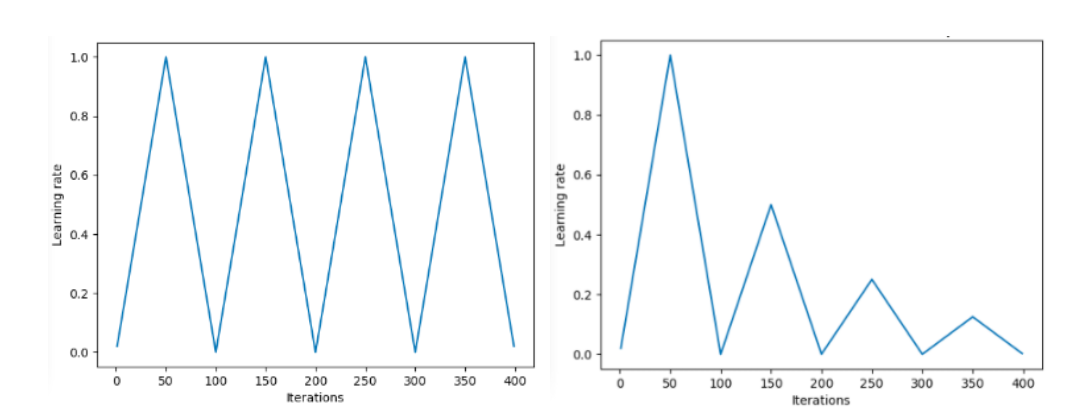
‘Triangular’ and ‘Triangular2’ methods for cycling learning rate proposed by Leslie N. Smith. On the left plot min and max lr are kept the same. On the right the difference is cut in half after each cycle. Image Credits: Hafidz Zulkifli
Something called stochastic gradient descent with warm restarts basically anneals the learning rate to a lower bound, and then restores the learning rate to it's original value.
We also have different schedules as to how the learning rates decline, from exponential decay to cosine decay.
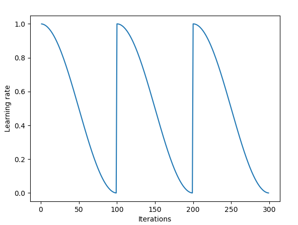
Cosine Annealing combined with restarts
A very recent paper introduces a technique called Stochastic Weight Averaging. The authors develop an approach where they first converge to a minima, cache the weights and then restore the learning rate to a higher value. This higher learning rate then propels the algorithm out of the minima to a random point in the loss surface. Then the algorithm is made to converge again to another minima. This is repeated for a few times. Finally, they average the predictions made by all the set of cached weights to produce the final prediction.
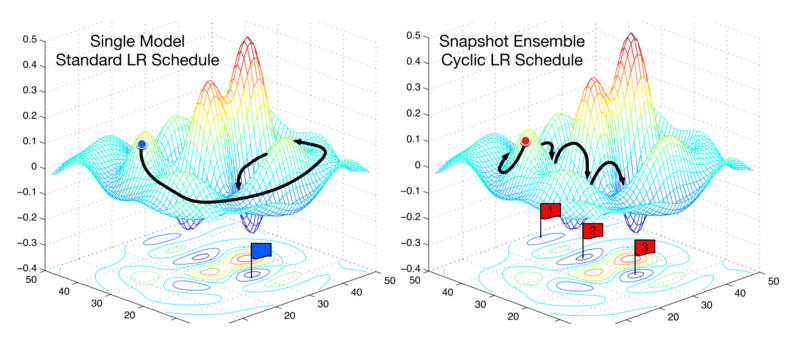
A technique called Stochastic Weight Averaging
Conclusion
So, this was the introductory post on gradient descent, that has been the working horse for deep learning optimization since the seminal paper on backpropogation that showed you could train neural nets by computing gradients. However, there's still one missing block about Gradient descent that we haven't talked about in this post, and that is addressing the problem of pathological curvature. Extensions to vanilla Stochastic Gradient Descent, like Momentum, RMSProp and Adam are used to overcome that vital problem.
However, I think whatever we have done is enough for one post, and the rest of it will be covered in another post.
Further Reading
1. Visual Loss Landscapes For Neural Nets (Paper)
2. A Brilliant Article on Learning Rate Schedules by Hafidz Zulkifli.