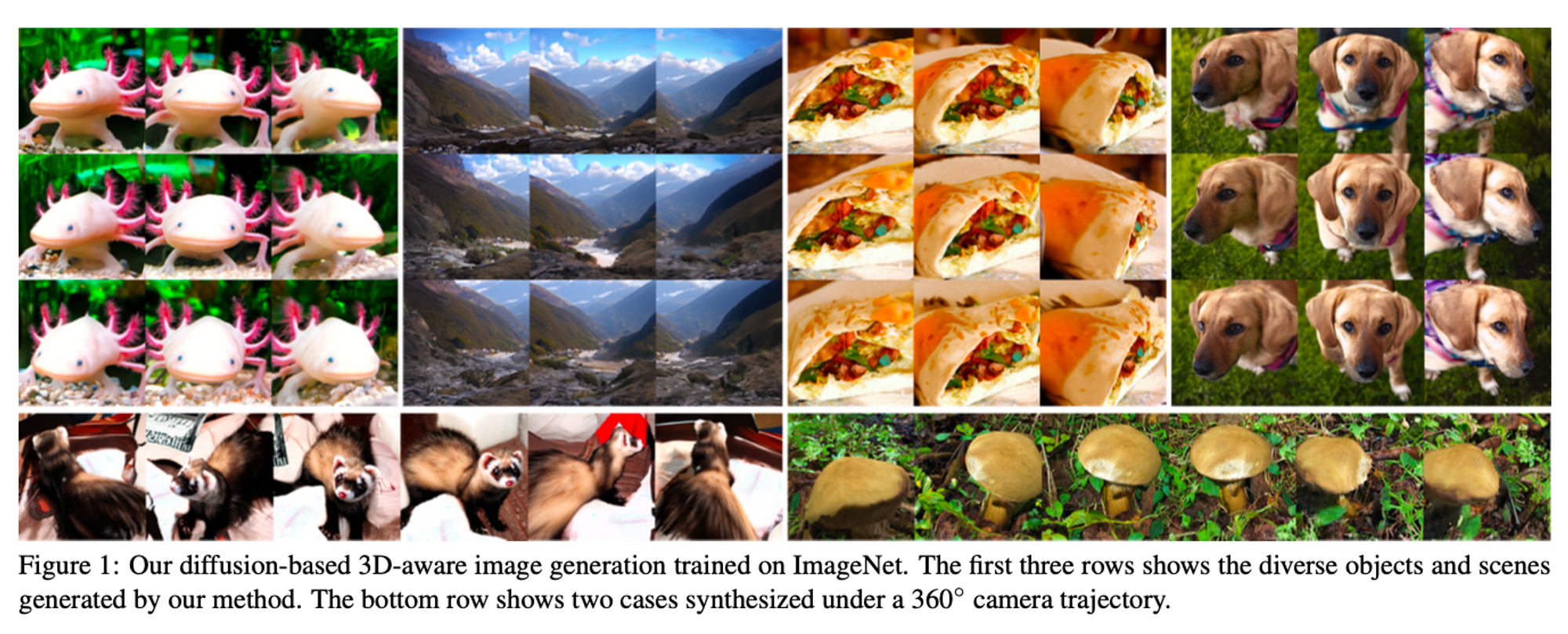
3D image generation models work by explicitly controlling the 3D camera pose. The majority of the 3D models work by exploiting 2D image datasets due to the scarcity of large-scale 3D datasets. Diffusion models are currently the state-of-art architecture for image generation but generating 3D data is a difficult task.
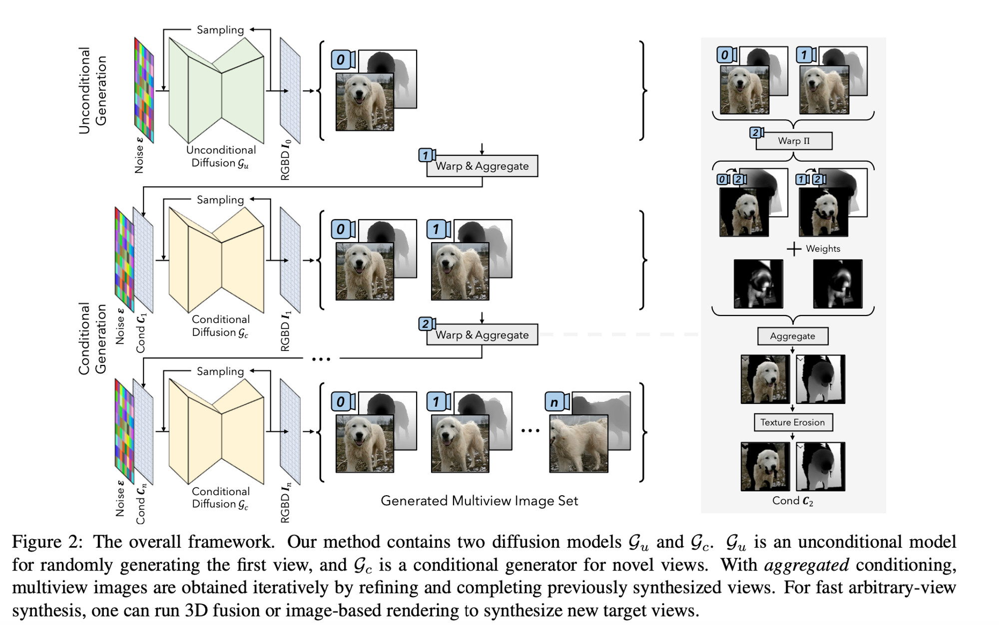
One reason for this is the lack of ample 3D asset datasets and the complexity of generating a set of related images from a diffusion model. In this paper, they propose viewing the task of set generation as a sequential unconditional-conditional generation process. They do this by sampling the initial view of an instance using an unconditional diffusion model and then iteratively sampling other views with previous views as conditions.
The challenge of a lack of adequate multi-view data is addressed by creating new images by appending depth information to image data through monocular depth estimation techniques. In addition to appending depth information, they implement additional data augmentation strategies to improve the generation quality.
Diffusion Models Recap
We know that diffusion models are trained using a forward noising process and a reverse denoising process. In the forward process, the model adds a fixed amount of Gaussian noise to the training data in a linear fashion while in the reverse process, the model predicts the amount of noise added to the given input data and subtracts the predicted noise to recover a ‘cleaner’ image. During inference, the denoising network employs the reverse denoising process to recover an image sample. A conditional diffusion model employs the same networks but also includes a condition $c$ to the target data distributions.
3D Generation as Iterative View Sampling
The authors work on the assumption that the distribution of 3D assets, denoted as $q_a(x)$, is equivalent to the joint distribution of its corresponding multiview images. Given a sequence of camera positions $\{ \pi_0, \pi_1, \pi_2..., \pi_N\}$ we can predict the given image using the camera position $\pi_*$ as a condition.
“$q_a(x) = q_i(\Gamma(x,\pi_0),\Gamma(x,\pi_1),...,\Gamma(x,\pi_N))$ , where $q_i$ is the distribution of images observed from 3D assets, and $\Gamma(.,.)$ is the 3D-2D rendering operator.” (paper) In this equation you can see that the joint distribution is derived from sampling several images from different camera positions to get the different viewpoints. When the images from this distribution are viewed together they create a 3D representation of the object or scene.
The joint distribution can also be represented as a series of conditioned distributions. This version is more intuitive because each sampling $\Gamma(x,\pi_n)$ takes in the previous samples as conditions — this ensures that there is little to no information gap when moving from one camera position to another; it’s almost as if it happens smoothly as the transition is from camera positions/viewpoints that are close to each other.
Because multi-view images are difficult to obtain, the authors use unstructured 2D image collections to construct the training data using image warping. This is done by “substituting the original condition images $\{\Gamma(x,\pi_k) k=1,...,n-1\}$ for $\Gamma(x,\pi_n)$ as $\Pi(\Gamma(x,\pi_k),\pi_n)$, where $\Pi(.,.)$ denotes the depth-based image warping operation that warps an image to a given target view using depth.” Using this new technique they eliminate the need for actual multiview images by warping the original image $\Gamma(x,\pi_n)$ back and forth. The authors regard the new distribution $q_d$ as $q_i(\Gamma(x,\pi_0))$ which is the distribution of 3D assets’ first partial view. All other views are relative to the first view. An unconditional model is trained on the first view $q_i(\Gamma(x,\pi_0))$ , and a conditional model is trained for other views $qi(\Gamma(x,\pi_n)|\Pi(\Gamma(x,\pi_0)\pi_n),...)$.
How Did They Prepare Their Data?
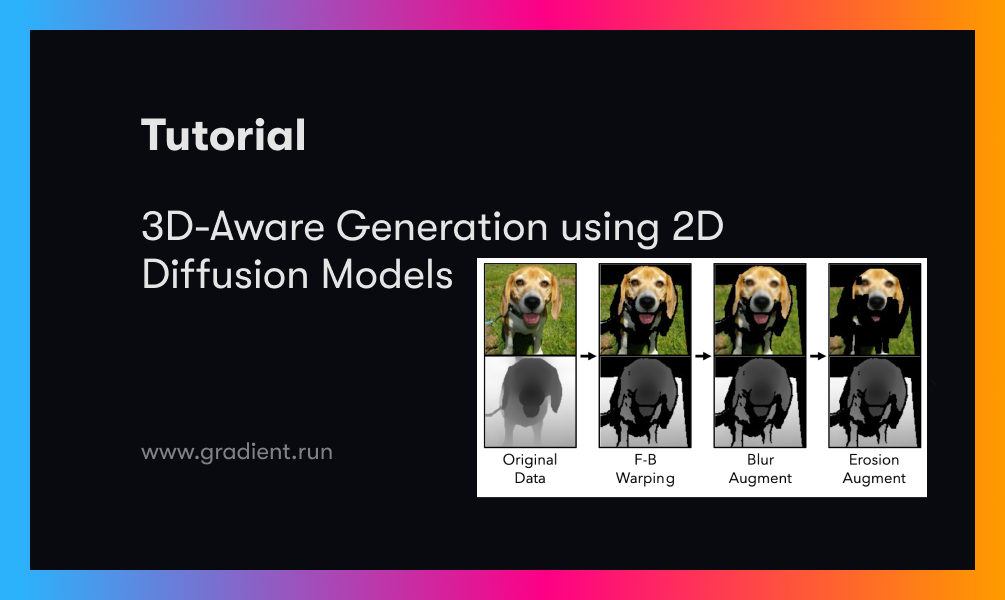
Most papers generally outline the contents of their datasets but this paper went in-depth (no pun intended) to describe their data preparation process because it solves a critical challenge in 3D image generation; lack of adequate training data. To start, they used the [actual name] monocular depth estimator to predict a depth map for each image in their starting dataset. Thereafter they apply an “RGBD-warping operator” to determine the relevant information of partial RGBD observations under novel viewpoints. This is done by taking in an image and target camera as input and then outputting the visible image contents under the target view as well as a visibility mask.
In order to construct the pairs of training images for conditional generation, they adopt a forward-backward warping strategy to construct the training pairs from a single image. Using this strategy the target RGBD images are first warped to novel views and then warped back to the original target views.
How Did They Train The Model?
They train both an unconditional and conditional model. They train an unconditional diffusion model to handle the distribution of all 2D RGBD images that were created by the warping operation. They adapt the ADM network architecture to handle the depth channel and they use classifier-free guidance with a dropping rate of 10% to handle the class labels. The unconditional model generated the first image in the sequence of multiview images for a given object.
They train a conditional model to generate sequential views after establishing the base view output by the unconditional model. The constructed data pairs that used the forward-backward warping strategy (introduced in the data prep section) are used here in the conditional model. In order to make the model more generalizable, they randomly sample the camera parameters $\pi$ from the Gaussian distribution as opposed to presenting the model with sequential camera poses. Tom combines the output from the unconditional model, the authors concatenate the original noisy image with the warped RGBD image with a mask to form the input to the conditional model. Classifier-free guidance is not applied to these conditions. In order to ensure model robustness, they apply several data augmentation strategies i.e. blur augmentation and texture erosion augmentation.
How Can We Make Inferences
Once the conditional and unconditional diffusion models have been trained we can go ahead and sample multi-view images. The first step is to define the sequence of camera poses that covers the desired views for multi-view synthesis. Given this camera sequence, novel views are generated sequentially with previously sampled images as conditions. In order to ensure that the current condition incorporates previous samples they use aggregated sampling. Aggregated conditioning collects information from previous images by performing a weighted sum across all warped versions of the previous images.
Summary
At the time of writing this article, the code for this model is not publicly available. However, certain portions of the architecture can be implemented from pre-existing models i.e the data prep can be done using the image warping operator (Ranftl, René, et al.) and the unconditional RGBD model could potentially train a custom DPM on the data you have prepared. There are several applications of this model in training 3D diffusion models on rare assets that only exist in a few 2D images.
Citations
- Xiang, Jianfeng, et al. "3D-aware Image Generation using 2D Diffusion Models." arXiv preprint arXiv:2303.17905 (2023).
- Ranftl, René, et al. "Towards robust monocular depth estimation: Mixing datasets for zero-shot cross-dataset transfer." IEEE transactions on pattern analysis and machine intelligence 44.3 (2020): 1623-1637.