Writing AlexNet from Scratch in PyTorch

This post is in continuation of my series of building classical and most popular convolutional neural networks from scratch in PyTorch. You can see the previous post here, where we built LeNet5. In this post, we will build AlexNet, one of the most popular and earliest breakthrough algorithms in Computer Vision.

We will start by investigating and understanding the architecture of AlexNet. We will then dive straight into code by loading our dataset, CIFAR10, before jumping in by applying some pre-processing to the data. Then, we will build our AlexNet from scratch using PyTorch and train it on our pre-processed data. The trained model will be tested on unseen (test) data for evaluation purposes at the end

AlexNet

AlexNet is a deep convolutional neural network, which was initially developed by Alex Krizhevsky and his colleagues back in 2012. It was designed to classify images for the ImageNet LSVRC-2010 competition where it achieved state of the art results. You can read in detail about the model in the original research paper here.

Here, I'll summarize the key takeaways about the AlexNet network. Firstly, it operated with 3-channel images that were (224x224x3) in size. It used max pooling along with ReLU activations when subsampling. The kernels used for convolutions were either 11x11, 5x5, or 3x3 while kernels used for max pooling were 3x3 in size. It classified images into 1000 classes. It also utilized multiple GPUs.

Data Loading

Dataset

Let's start by loading and then pre-processing the data. For our purposes, we will be using the CIFAR10 dataset. The dataset consists of 60000 32x32 colour images in 10 classes, with 6000 images per class. There are 50000 training images and 10000 test images.

Here are the classes in the dataset, as well as 10 random sample images from each:

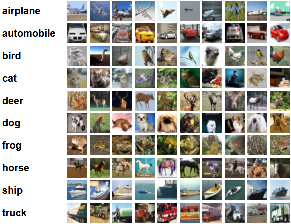
The classes are completely mutually exclusive. There is no overlap between automobiles and trucks. "Automobile" includes sedans, SUVs, and things of that sort. "Truck" includes only big trucks. Neither includes pickup trucks.

Importing the Libraries

Let's start by importing the required libraries along with defining a variable device, so that the Notebook knows to use a GPU to train the model if it's available.

import numpy as np
import torch
import torch.nn as nn
from torchvision import datasets
from torchvision import transforms
from torch.utils.data.sampler import SubsetRandomSampler


# Device configuration
device = torch.device('cuda' if torch.cuda.is_available() else 'cpu')

Loading the Dataset

Using torchvision (a helper library for computer vision tasks), we will load our dataset. This method has some helper functions that makes pre-processing pretty easy and straight-forward. Let's define the functions get_train_valid_loader and get_test_loader, and then call them to load in and process our CIFAR-10 data:

def get_train_valid_loader(data_dir,
                           batch_size,
                           augment,
                           random_seed,
                           valid_size=0.1,
                           shuffle=True):
    normalize = transforms.Normalize(
        mean=[0.4914, 0.4822, 0.4465],
        std=[0.2023, 0.1994, 0.2010],
    )

    # define transforms
    valid_transform = transforms.Compose([
            transforms.Resize((227,227)),
            transforms.ToTensor(),
            normalize,
    ])
    if augment:
        train_transform = transforms.Compose([
            transforms.RandomCrop(32, padding=4),
            transforms.RandomHorizontalFlip(),
            transforms.ToTensor(),
            normalize,
        ])
    else:
        train_transform = transforms.Compose([
            transforms.Resize((227,227)),
            transforms.ToTensor(),
            normalize,
        ])

    # load the dataset
    train_dataset = datasets.CIFAR10(
        root=data_dir, train=True,
        download=True, transform=train_transform,
    )

    valid_dataset = datasets.CIFAR10(
        root=data_dir, train=True,
        download=True, transform=valid_transform,
    )

    num_train = len(train_dataset)
    indices = list(range(num_train))
    split = int(np.floor(valid_size * num_train))

    if shuffle:
        np.random.seed(random_seed)
        np.random.shuffle(indices)

    train_idx, valid_idx = indices[split:], indices[:split]
    train_sampler = SubsetRandomSampler(train_idx)
    valid_sampler = SubsetRandomSampler(valid_idx)

    train_loader = torch.utils.data.DataLoader(
        train_dataset, batch_size=batch_size, sampler=train_sampler)
 
    valid_loader = torch.utils.data.DataLoader(
        valid_dataset, batch_size=batch_size, sampler=valid_sampler)

    return (train_loader, valid_loader)


def get_test_loader(data_dir,
                    batch_size,
                    shuffle=True):
    normalize = transforms.Normalize(
        mean=[0.485, 0.456, 0.406],
        std=[0.229, 0.224, 0.225],
    )

    # define transform
    transform = transforms.Compose([
        transforms.Resize((227,227)),
        transforms.ToTensor(),
        normalize,
    ])

    dataset = datasets.CIFAR10(
        root=data_dir, train=False,
        download=True, transform=transform,
    )

    data_loader = torch.utils.data.DataLoader(
        dataset, batch_size=batch_size, shuffle=shuffle
    )

    return data_loader


# CIFAR10 dataset 
train_loader, valid_loader = get_train_valid_loader(data_dir = './data',                                      batch_size = 64,
                       augment = False,                             		     random_seed = 1)

test_loader = get_test_loader(data_dir = './data',
                              batch_size = 64)

Let's break down the code into bits:

• We define two functions get_train_valid_loader and get_test_loader to load train/validation and test sets respectively
• We start by defining the variable normalize with the mean and standard deviations of each of the channel (red, green, and blue) in the dataset. These can be calculated manually, but are also available online since CIFAR-10 is quite popular
• For our training dataset, we add the option to augment the dataset as well for more robust training and increasing the number of images as well. Note: augmentation is only applied to the training subset and not the validation and testing subsets as they are only used for evaluation purposes
• We split the training dataset into train and validation sets (90:10 ratio), and randomly subset it from the whole training set
• We specify the batch size and shuffle the dataset when loading, so that every batch has some variance in the types of labels it has. This will increase the efficacy of our eventual model
• Finally, we make use of data loaders. This might not affect the performance in the case of a small dataset like CIFAR10, but it can really impede the performance in case of large datasets and is generally considered a good practice. Data loaders allow us to iterate through the data in batches, and the data is loaded while iterating and not all at once in start into your RAM

AlexNet from Scratch

Let's start with the code first:

class AlexNet(nn.Module):
    def __init__(self, num_classes=10):
        super(AlexNet, self).__init__()
        self.layer1 = nn.Sequential(
            nn.Conv2d(3, 96, kernel_size=11, stride=4, padding=0),
            nn.BatchNorm2d(96),
            nn.ReLU(),
            nn.MaxPool2d(kernel_size = 3, stride = 2))
        self.layer2 = nn.Sequential(
            nn.Conv2d(96, 256, kernel_size=5, stride=1, padding=2),
            nn.BatchNorm2d(256),
            nn.ReLU(),
            nn.MaxPool2d(kernel_size = 3, stride = 2))
        self.layer3 = nn.Sequential(
            nn.Conv2d(256, 384, kernel_size=3, stride=1, padding=1),
            nn.BatchNorm2d(384),
            nn.ReLU())
        self.layer4 = nn.Sequential(
            nn.Conv2d(384, 384, kernel_size=3, stride=1, padding=1),
            nn.BatchNorm2d(384),
            nn.ReLU())
        self.layer5 = nn.Sequential(
            nn.Conv2d(384, 256, kernel_size=3, stride=1, padding=1),
            nn.BatchNorm2d(256),
            nn.ReLU(),
            nn.MaxPool2d(kernel_size = 3, stride = 2))
        self.fc = nn.Sequential(
            nn.Dropout(0.5),
            nn.Linear(9216, 4096),
            nn.ReLU())
        self.fc1 = nn.Sequential(
            nn.Dropout(0.5),
            nn.Linear(4096, 4096),
            nn.ReLU())
        self.fc2= nn.Sequential(
            nn.Linear(4096, num_classes))
        
    def forward(self, x):
        out = self.layer1(x)
        out = self.layer2(out)
        out = self.layer3(out)
        out = self.layer4(out)
        out = self.layer5(out)
        out = out.reshape(out.size(0), -1)
        out = self.fc(out)
        out = self.fc1(out)
        out = self.fc2(out)
        return out

Let's dive into how the above code works:

• The first step to defining any neural network (whether a CNN or not) in PyTorch is to define a class that inherits nn.Module as it contains many of the methods that we will need to utilize
• There are two main steps after that. First is initializing the layers that we are going to use in our CNN inside __init__ , and the other is to define the sequence in which those layers will process the image. This is defined inside the forward function
• For the architecture itself, we first define the convolutional layers using the nn.Conv2D function with the appropriate kernel size and the input/output channels. We also apply max pooling using nn.MaxPool2D function. The nice thing about PyTorch is that we can combine the convolutional layer, activation function, and max pooling into one single layer (they will be separately applied, but it helps with organization) using the nn.Sequential function
• Then we define the fully connected layers using linear (nn.Linear) and dropout (nn.Dropout) along with ReLu activation function (nn.ReLU) and combining these with the nn.Sequential function
• Finally, our last layer outputs 10 neurons which are our final predictions for the 10 classes of objects

Setting Hyperparameters

Before training, we need to set some hyperparameters, such as the loss function and the optimizer to be used along with batch size, learning rate, and number of epochs.

num_classes = 10
num_epochs = 20
batch_size = 64
learning_rate = 0.005

model = AlexNet(num_classes).to(device)


# Loss and optimizer
criterion = nn.CrossEntropyLoss()
optimizer = torch.optim.SGD(model.parameters(), lr=learning_rate, weight_decay = 0.005, momentum = 0.9)  


# Train the model
total_step = len(train_loader)

We start by defining simple hyperparameters (epochs, batch size, and learning rate) and initializing our model using the number of classes as an argument, which in this case is 10 along with transferring the model to the appropriate device (CPU or GPU). Then we define our cost function as cross entropy loss and optimizer as Adam. There are a lot of choices for these, but these tend to give good results with the model and the given data. Finally, we define total_step to keep better track of steps when training

Training

We are ready to train our model at this point:

total_step = len(train_loader)

for epoch in range(num_epochs):
    for i, (images, labels) in enumerate(train_loader):  
        # Move tensors to the configured device
        images = images.to(device)
        labels = labels.to(device)
        
        # Forward pass
        outputs = model(images)
        loss = criterion(outputs, labels)
        
        # Backward and optimize
        optimizer.zero_grad()
        loss.backward()
        optimizer.step()

    print ('Epoch [{}/{}], Step [{}/{}], Loss: {:.4f}' 
                   .format(epoch+1, num_epochs, i+1, total_step, loss.item()))
            
    # Validation
    with torch.no_grad():
        correct = 0
        total = 0
        for images, labels in valid_loader:
            images = images.to(device)
            labels = labels.to(device)
            outputs = model(images)
            _, predicted = torch.max(outputs.data, 1)
            total += labels.size(0)
            correct += (predicted == labels).sum().item()
            del images, labels, outputs
    
        print('Accuracy of the network on the {} validation images: {} %'.format(5000, 100 * correct / total)) 

Let's see what the code does:

• We start by iterating through the number of epochs, and then the batches in our training data
• We convert the images and the labels according to the device we are using, i.e., GPU or CPU
• In the forward pass, we make predictions using our model and calculate loss based on those predictions and our actual labels
• Next, we do the backward pass where we actually update our weights to improve our model
• We then set the gradients to zero before every update using optimizer.zero_grad() function
• Then, we calculate the new gradients using the loss.backward() function
• And finally, we update the weights with the optimizer.step() function
• Also, at the end of every epoch we use our validation set to calculate the accuracy of the model as well. In this case, we don't need gradients so we use with torch.no_grad() for faster evaluation

We can see the output as follows:

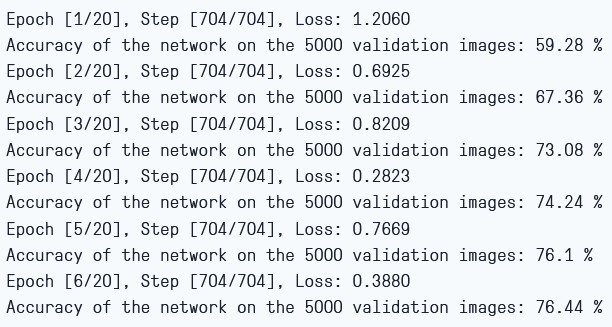
As we can see, the loss is decreasing with every epoch which shows that our model is indeed learning. Note that this loss is on the training set, and if the loss is way too small it can indicate overfitting. This is why we are using the validation set as well. The accuracy seems to be increasing on validation set which indicates that there is an unlikely chance of any overfitting. Let's now test our model to see how it performs.

Testing

Now, we see how our model performs on unseen data:

with torch.no_grad():
    correct = 0
    total = 0
    for images, labels in test_loader:
        images = images.to(device)
        labels = labels.to(device)
        outputs = model(images)
        _, predicted = torch.max(outputs.data, 1)
        total += labels.size(0)
        correct += (predicted == labels).sum().item()
        del images, labels, outputs

    print('Accuracy of the network on the {} test images: {} %'.format(10000, 100 * correct / total))   

Note that the code is exactly the same as for our validation purposes.

Using the model, and training for only 6 epochs, we seem to get around 78.8% accuracy on the validation set which seems good enough

Conclusion

Let's now conclude what we did in this article:

• We started by understanding the architecture and different kinds of layers in the AlexNet model
• Next, we loaded and pre-processed the CIFAR10 dataset using torchvision
• Then, we used PyTorch to build our AlexNet model from scratch
• Finally, we trained and tested our model on the CIFAR10 dataset, and the model seemed to perform well on the test dataset with minimal training (6 epochs)

Future Work

Using this article, you get a good introduction and hand-on learning but you'll learn much more if you extend this and see what you can do else:

• You can try using different datasets. One such dataset is CIFAR100 which is an extension of the CIFAR10 dataset with 100 classes
• You can experiment with different hyperparameters and see the best combination of them for the model
• Finally, you can try adding or removing layers from the dataset to see their impact on the capability of the model

To run this on Gradient Notebooks, simply put this URL in the advanced options boxed marked "Workspace URL." This is the GitHub repo for this article.