As a follow-up to my previous post, we will continue writing convolutional neural networks from scratch in PyTorch by building some of the classic CNNs and see them in action on a dataset.
Introduction
In this article, we will be building one of the earliest Convolutional Neural Networks ever introduced, LeNet5 (paper). We are building this CNN from scratch in PyTorch, and will also see how it performs on a real-world dataset.
We will start by exploring the architecture of LeNet5. We will then load and analyze our dataset, MNIST, using the provided class from torchvision. Using PyTorch, we will build our LeNet5 from scratch and train it on our data. Finally, we will see how the model performs on the unseen test data.
LeNet5
LeNet5 is one of the earliest Convolutional Neural Networks (CNNs). It was proposed by Yann LeCun and others in 1998. You can read the original paper here: Gradient-Based Learning Applied to Document Recognition. In the paper, the LeNet5 was used for the recognition of handwritten characters.
Let's now understand the architecture of LeNet5 as shown in the figure below:
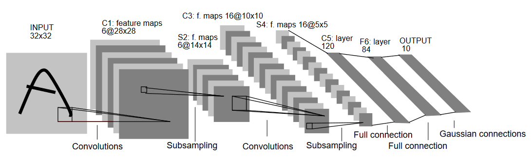
As the name indicates, LeNet5 has 5 layers with two convolutional and three fully connected layers. Let's start with the input. LeNet5 accepts as input a greyscale image of 32x32, indicating that the architecture is not suitable for RGB images (multiple channels). So the input image should contain just one channel. After this, we start with our convolutional layers
The first convolutional layer has a filter size of 5x5 with 6 such filters. This will reduce the width and height of the image while increasing the depth (number of channels). The output would be 28x28x6. After this, pooling is applied to decrease the feature map by half, i.e, 14x14x6. Same filter size (5x5) with 16 filters is now applied to the output followed by a pooling layer. This reduces the output feature map to 5x5x16.
After this, a convolutional layer of size 5x5 with 120 filters is applied to flatten the feature map to 120 values. Then comes the first fully connected layer, with 84 neurons. Finally, we have the output layer which has 10 output neurons, since the MNIST data have 10 classes for each of the represented 10 numerical digits.
Data Loading
Dataset
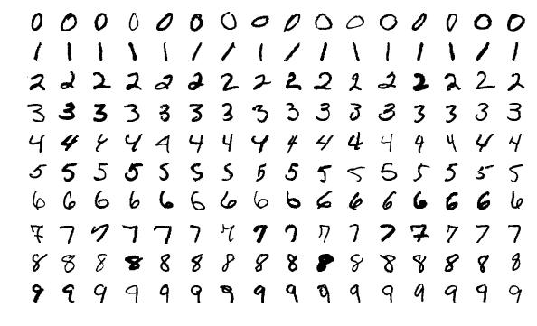
Let's start by loading and analyzing the data. We will be using the MNIST dataset. The MNIST dataset contains images of handwritten numerical digits. The images are greyscale, all with a size of 28x28, and is composed of 60,000 training images and 10,000 testing images.
You can see some of the samples of images below:
Importing the Libraries
Let's start by importing the required libraries and defining some variables (hyperparameters and device are also detailed to help the package determine whether to train on GPU or CPU):
# Load in relevant libraries, and alias where appropriate
import torch
import torch.nn as nn
import torchvision
import torchvision.transforms as transforms

# Define relevant variables for the ML task
batch_size = 64
num_classes = 10
learning_rate = 0.001
num_epochs = 10

# Device will determine whether to run the training on GPU or CPU.
device = torch.device('cuda' if torch.cuda.is_available() else 'cpu')Loading the Dataset
Using torchvision , we will load the dataset as this will allow us to perform any pre-processing steps easily.
#Loading the dataset and preprocessing
train_dataset = torchvision.datasets.MNIST(root = './data',
                                           train = True,
                                           transform = transforms.Compose([
                                                  transforms.Resize((32,32)),
                                                  transforms.ToTensor(),
                                                  transforms.Normalize(mean = (0.1307,), std = (0.3081,))]),
                                           download = True)


test_dataset = torchvision.datasets.MNIST(root = './data',
                                          train = False,
                                          transform = transforms.Compose([
                                                  transforms.Resize((32,32)),
                                                  transforms.ToTensor(),
                                                  transforms.Normalize(mean = (0.1325,), std = (0.3105,))]),
                                          download=True)


train_loader = torch.utils.data.DataLoader(dataset = train_dataset,
                                           batch_size = batch_size,
                                           shuffle = True)


test_loader = torch.utils.data.DataLoader(dataset = test_dataset,
                                           batch_size = batch_size,
shuffle = True)Let's understand the code:
- Firstly, the MNIST data can't be used as it is for the LeNet5 architecture. The LeNet5 architecture accepts the input to be 32x32 and the MNIST images are 28x28. We can fix this by resizing the images, normalizing them using the pre-calculated mean and standard deviation (available online), and finally storing them as tensors.
- We set
download=Trueincase the data is not already downloaded. - Next, we make use of data loaders. This might not affect the performance in the case of a small dataset like MNIST, but it can really impede the performance in case of large datasets and is generally considered a good practice. Data loaders allow us to iterate through the data in batches, and the data is loaded while iterating and not at once in start.
- We specify the batch size and shuffle the dataset when loading so that every batch has some variance in the types of labels it has. This will increase the efficacy of our eventual model.
Bring this project to life
LeNet5 from Scratch
Let's first look into the code:
#Defining the convolutional neural network
class LeNet5(nn.Module):
    def __init__(self, num_classes):
        super(ConvNeuralNet, self).__init__()
        self.layer1 = nn.Sequential(
            nn.Conv2d(1, 6, kernel_size=5, stride=1, padding=0),
            nn.BatchNorm2d(6),
            nn.ReLU(),
            nn.MaxPool2d(kernel_size = 2, stride = 2))
        self.layer2 = nn.Sequential(
            nn.Conv2d(6, 16, kernel_size=5, stride=1, padding=0),
            nn.BatchNorm2d(16),
            nn.ReLU(),
            nn.MaxPool2d(kernel_size = 2, stride = 2))
        self.fc = nn.Linear(400, 120)
        self.relu = nn.ReLU()
        self.fc1 = nn.Linear(120, 84)
        self.relu1 = nn.ReLU()
        self.fc2 = nn.Linear(84, num_classes)

    def forward(self, x):
        out = self.layer1(x)
        out = self.layer2(out)
        out = out.reshape(out.size(0), -1)
        out = self.fc(out)
        out = self.relu(out)
        out = self.fc1(out)
        out = self.relu1(out)
        out = self.fc2(out)
return outI'll explain the code linearly:
- In PyTorch, we define a neural network by creating a class that inherits from
nn.Moduleas it contains many of the methods that we will need to utilize. - There are two main steps after that. First is initializing the layers that we are going to use in our CNN inside
__init__, and the other is to define the sequence in which those layers will process the image. This is defined inside theforwardfunction. - For the architecture itself, we first define the convolutional layers using the
nn.Conv2Dfunction with the appropriate kernel size and the input/output channels. We also apply max pooling usingnn.MaxPool2Dfunction. The nice thing about PyTorch is that we can combine the convolutional layer, activation function, and max pooling into one single layer (they will be separately applied, but it helps with organization) using thenn.Sequentialfunction. - Then we define the fully connected layers. Note that we can use
nn.Sequentialhere as well and combine the activation functions and the linear layers, but I wanted to show that either one is possible. - Finally, our last layer outputs 10 neurons which are our final predictions for the digits.
Setting Hyperparameters
Before training, we need to set some hyperparameters, such as the loss function and the optimizer to be used.
model = LeNet5(num_classes).to(device)

#Setting the loss function
cost = nn.CrossEntropyLoss()

#Setting the optimizer with the model parameters and learning rate
optimizer = torch.optim.Adam(model.parameters(), lr=learning_rate)

#this is defined to print how many steps are remaining when training
total_step = len(train_loader)We start by initializing our model using the number of classes as an argument, which in this case is 10. Then we define our cost function as cross entropy loss and optimizer as Adam. There are a lot of choices for these, but these tend to give good results with the model and the given data. Finally, we define total_step to keep better track of steps when training.
Training
Now, we can train our model:
total_step = len(train_loader)
for epoch in range(num_epochs):
    for i, (images, labels) in enumerate(train_loader):
        images = images.to(device)
        labels = labels.to(device)

        #Forward pass
        outputs = model(images)
        loss = cost(outputs, labels)

        # Backward and optimize
        optimizer.zero_grad()
        loss.backward()
        optimizer.step()

        if (i+1) % 400 == 0:
            print ('Epoch [{}/{}], Step [{}/{}], Loss: {:.4f}'
.format(epoch+1, num_epochs, i+1, total_step, loss.item()))Let's see what the code does:
- We start by iterating through the number of epochs, and then the batches in our training data.
- We convert the images and the labels according to the device we are using, i.e., GPU or CPU.
- In the forward pass, we make predictions using our model and calculate loss based on those predictions and our actual labels.
- Next, we do the backward pass where we actually update our weights to improve our model
- We then set the gradients to zero before every update using
optimizer.zero_grad()function. - Then, we calculate the new gradients using the
loss.backward()function. - And finally, we update the weights with the
optimizer.step()function.
We can see the output as follows:
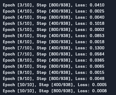
As we can see, the loss is decreasing with every epoch which shows that our model is indeed learning. Note that this loss is on the training set, and if the loss is way too small (as is in our case), it can indicate overfitting. There are multiple ways to solve that problem such as regularization, data augmentation, and so on but we won't be getting into that in this article. Let's now test our model to see how it performs.
Testing
Let's now test our model:
# Test the model
# In test phase, we don't need to compute gradients (for memory efficiency)

with torch.no_grad():
    correct = 0
    total = 0
    for images, labels in test_loader:
        images = images.to(device)
        labels = labels.to(device)
        outputs = model(images)
        _, predicted = torch.max(outputs.data, 1)
        total += labels.size(0)
        correct += (predicted == labels).sum().item()

    print('Accuracy of the network on the 10000 test images: {} %'.format(100 * correct / total))
As you can see, the code is not so different than the one for training. The only difference is that we are not computing gradients (using with torch.no_grad()), and also not computing the loss because we don't need to backpropagate here. To compute the resulting accuracy of the model, we can simply calculate the total number of correct predictions over the total number of images.
Using this model, we get around 98.8% accuracy which is quite good:

Note that MNIST dataset is quite basic and small for today's standards, and similar results are hard to get for other datasets. Nonetheless, it's a good starting point when learning deep learning and CNNs.
Conclusion
Let's now conclude what we did in this article:
- We started by learning the architecture of LeNet5 and the different kinds of layers in that.
- Next, we explored the MNIST dataset and loaded the data using
torchvision. - Then, we built LeNet5 from scratch along with defining hyperparameters for the model.
- Finally, we trained and tested our model on the MNIST dataset, and the model seemed to perform well on the test dataset.
Future Work
Although this seems a really good introduction to deep learning in PyTorch, you can extend this work to learn more as well:
- You can try using different datasets but for this model you will need gray scale datasets. One such dataset is FashionMNIST.
- You can experiment with different hyperparameters and see the best combination of them for the model.
- Finally, you can try adding or removing layers from the dataset to see their impact on the capability of the model.
Find the Github repo for this tutorial here: https://github.com/gradient-ai/LeNet5-Tutorial