Image Compression Using Autoencoders in Keras

Autoencoders are a deep learning model for transforming data from a high-dimensional space to a lower-dimensional space. They work by encoding the data, whatever its size, to a 1-D vector. This vector can then be decoded to reconstruct the original data (in this case, an image). The more accurate the autoencoder, the closer the generated data is to the original.

In this tutorial we'll explore the autoencoder architecture and see how we can apply this model to compress images from the MNIST dataset using TensorFlow and Keras. In particular, we'll consider:

• Discriminative vs. Generative Modeling
• How Autoencoders Work
• Building an Autoencoder in Keras
  • Building the Encoder
  • Building the Decoder
• Training
• Making Predictions
• Complete Code
• Conclusion

Discriminative vs. Generative Modeling

The most common type of machine learning models are discriminative. If you're a machine learning enthusiast, it's likely that the type of models that you've built or used have been mainly discriminative. These models recognize the input data and then take appropriate action. For a classification task, a discriminative model learns how to differentiate between various different classes. Based on the model's learning about the properties of each class, it classifies a new input sample to the appropriate label. Let's apply this understanding to the next image representing a warning sign.

If a machine/deep learning model is to recognize the following image, it may understand that it consists of three main elements: a rectangle, a line, and a dot. When another input image has features which resemble these elements, then it should also be recognized as a warning sign.

If the algorithm is able to identify the properties of an image, could it generate a new image similar to it? In other words, could it draw a new image that has a triangle, a line, and a dot? Unfortunately, discriminative models are not clever enough to draw new images even if they know the structure of these images. Let's take another example to make things clearer.

Assume there is someone that can recognize things well. For a given image, he/she can easily identify the salient properties and then classify the image. Is it a must that such a person will be able to draw such an image again? No. Some people cannot draw things. Discriminative models are like those people who can just recognize images, but could not draw them on their own.

In contrast with discriminative models, there is another group called generative models which can create new images. For a given input image, the output of a discriminative model is a class label; the output of a generative model is an image of the same size and similar appearance as the input image.

One of the simplest generative models is the autoencoder (AE for short), which is the focus of this tutorial.

How Autoencoders Work

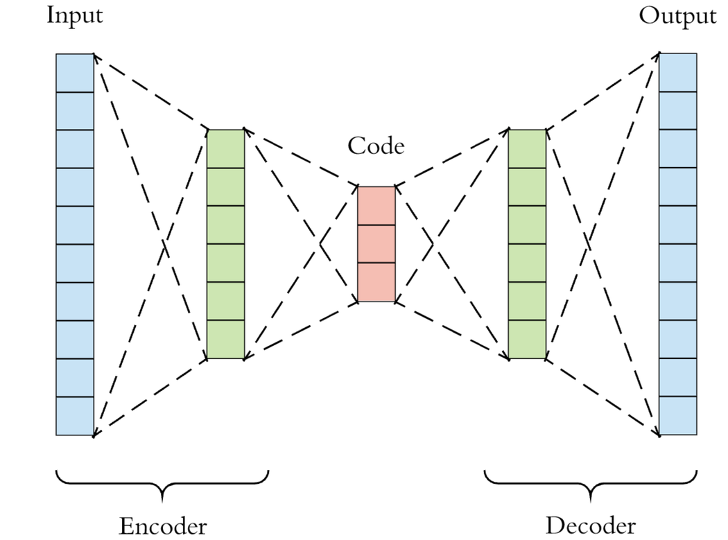
Autoencoders are a deep neural network model that can take in data, propagate it through a number of layers to condense and understand its structure, and finally generate that data again. In this tutorial we'll consider how this works for image data in particular. To accomplish this task an autoencoder uses two different types of networks. The first is called an encoder, and the other is the decoder. The decoder is just a reflection of the layers inside the encoder. Let's clarify how this works.

The job of the encoder is to accept the original data (e.g. an image) that could have two or more dimensions and generate a single 1-D vector that represents the entire image. The number of elements in the 1-D vector varies based on the task being solved. It could have 1 or more elements. The fewer elements in the vector, the more complexity in reproducing the original image accurately.

By representing the input image in a vector of relatively few elements, we actually compress the image. For example, the size of each image in the MNIST dataset (which we'll use in this tutorial) is 28x28. That is, each image has 784 elements. If each image is compressed so that it is represented using just two elements, then we spared 782 elements and thus (782/784)*100=99.745% of the data.

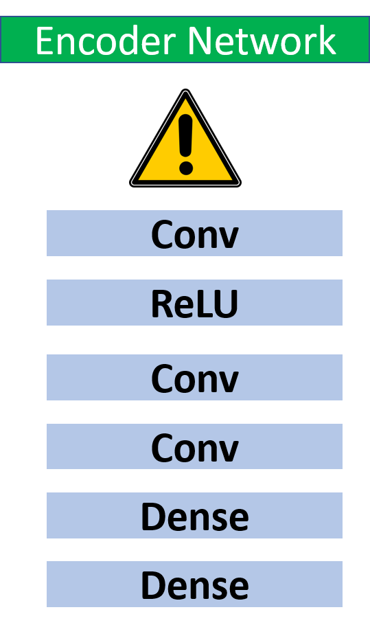
The next figure shows how an encoder generates the 1-D vector from an input image. The layers included are of your choosing, so you can use dense, convolutional, dropout, etc.

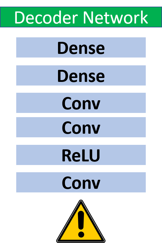
The 1-D vector generated by the encoder from its last layer is then fed to the decoder. The job of the decoder is to reconstruct the original image with the highest possible quality. The decoder is just a reflection of the encoder. According to the encoder architecture in the previous figure, the architecture of the decoder is given in the next figure.

The loss is calculated by comparing the original and reconstructed images, i.e. by calculating the difference between the pixels in the 2 images. Note that the output of the decoder must be of the same size as the original image. Why? Because if the size of the images is different, there is no way to calculate the loss.

After discussing how the autoencoder works, let's build our first autoencoder using Keras.

Building an Autoencoder in Keras

Keras is a powerful tool for building machine and deep learning models because it's simple and abstracted, so in little code you can achieve great results. Keras has three ways for building a model:

1. Sequential API
2. Functional API
3. Model Subclassing

The three ways differ in the level of customization allowed.

The sequential API allows you to build sequential models, but it is less customizable compared to the other two types. The output of each layer in the model is only connected to a single layer.

Although this is the type of model we want to create in this tutorial, we'll use the functional API. The functional API is simple, very similar to the sequential API, and also supports additional features such as the ability to connect the output of a single layer to multiple layers.

The last option for building a Keras model is model subclassing, which is fully-customizable but also very complex. You can read more about these three methods in this tutorial.

Now we'll focus on using the functional API for building the autoencoder. You might think that we are going  to build a single Keras model for representing the autoencoder, but we will actually build three models: one for the encoder, another for the decoder, and yet another for the complete autoencoder. Why do we build a model for both the encoder and the decoder? We do this in case you want to explore each model separately. For instance, we can use the model of the encoder to visualize the 1-D vector representing each input image, and this might help you to know whether it's a good representation of the image or not. With the decoder we'll be able to test whether good representations are being created from the 1-D vectors, assuming they are well-encoded (i.e. better for debugging purposes) Finally, by building a model for the entire autoencoder we can easily use it end-to-end by feeding it the original image and receiving the output image directly.

Let's start by building the encoder model.

Building the Encoder

The following code builds a model for the encoder using the functional API. At first, the layers of the model are created using the tensorflow.keras.layers API because we are using TensorFlow as the backend library. The first layer is an Input layer which accepts the original image. This layer accepts an argument named shape representing the size of the input, which depends on the dataset being used. We're going to use the MNIST dataset where the size of each image is 28x28. Rather than setting the shape to (28, 28), it's just set to (784). Why? Because we're going to use only dense layers in the network and thus the input must be in the form of a vector, not a matrix. The tensor representing the input layer is returned to the variable x.

The input layer is then propagated through a number of layers:

• Dense layer with 300 neurons
• LeakyReLU layer
• Dense layer with 2 neurons
• LeakyReLU layer

The last Dense layer in the network has just two neurons. When fed to the LeakyReLU layer, the final output of the encoder will be a 1-D vector with just two elements. In other words, all images in the MNIST dataset will be encoded as vectors of two elements.

import tensorflow.keras.layers
import tensorflow.keras.models

x = tensorflow.keras.layers.Input(shape=(784), name="encoder_input")

encoder_dense_layer1 = tensorflow.keras.layers.Dense(units=300, name="encoder_dense_1")(x)
encoder_activ_layer1 = tensorflow.keras.layers.LeakyReLU(name="encoder_leakyrelu_1")(encoder_dense_layer1)

encoder_dense_layer2 = tensorflow.keras.layers.Dense(units=2, name="encoder_dense_2")(encoder_activ_layer1)
encoder_output = tensorflow.keras.layers.LeakyReLU(name="encoder_output")(encoder_dense_layer2)

After building and connecting all of the layers, the next step is to build the model using the tensorflow.keras.models API by specifying the input and output tensors according to the next line:

encoder = tensorflow.keras.models.Model(x, encoder_output, name="encoder_model")

To print a summary of the encoder architecture we'll use encoder.summary(). The output is below. This network is not large and you can increase the number of neurons in the dense layer named encoder_dense_1 but I just used 300 neurons to avoid taking much time training the network.

_________________________________________________________________
Layer (type)                 Output Shape              Param #   
=================================================================
encoder_input (InputLayer)   [(None, 784)]             0         
_________________________________________________________________
encoder_dense_1 (Dense)      (None, 300)               235500    
_________________________________________________________________
encoder_leakyrelu_1 (LeakyRe (None, 300)               0         
_________________________________________________________________
encoder_dense_2 (Dense)      (None, 2)                 602       
_________________________________________________________________
encoder_output (LeakyReLU)   (None, 2)                 0         
=================================================================
Total params: 236,102
Trainable params: 236,102
Non-trainable params: 0
_________________________________________________________________

After building the encoder, next is to work on the decoder.

Building the Decoder

Similar to building the encoder, the decoder will be build using the following code. Because the input layer of the decoder accepts the output returned from the last layer in the encoder, we have to make sure these 2 layers match in the size. The last layer in the encoder returns a vector of 2 elements and thus the input of the decoder must have 2 neurons. You can easily note that the layers of the decoder are just reflection to those in the encoder.

decoder_input = tensorflow.keras.layers.Input(shape=(2), name="decoder_input")

decoder_dense_layer1 = tensorflow.keras.layers.Dense(units=300, name="decoder_dense_1")(decoder_input)
decoder_activ_layer1 = tensorflow.keras.layers.LeakyReLU(name="decoder_leakyrelu_1")(decoder_dense_layer1)

decoder_dense_layer2 = tensorflow.keras.layers.Dense(units=784, name="decoder_dense_2")(decoder_activ_layer1)
decoder_output = tensorflow.keras.layers.LeakyReLU(name="decoder_output")(decoder_dense_layer2)

After connecting the layers, next is to build the decoder model according to the next line.

decoder = tensorflow.keras.models.Model(decoder_input, decoder_output, name="decoder_model")

Here is the output of decoder.summary(). It is very important to make sure the size of the output returned from the encoder matches the original input size.

_________________________________________________________________
Layer (type)                 Output Shape              Param #   
=================================================================
decoder_input (InputLayer)   [(None, 2)]               0         
_________________________________________________________________
decoder_dense_1 (Dense)      (None, 300)               900       
_________________________________________________________________
decoder_leakyrelu_1 (LeakyRe (None, 300)               0         
_________________________________________________________________
decoder_dense_2 (Dense)      (None, 784)               235984    
_________________________________________________________________
decoder_output (LeakyReLU)   (None, 784)               0         
=================================================================
Total params: 236,884
Trainable params: 236,884
Non-trainable params: 0
_________________________________________________________________

After building the 2 blocks of the autoencoder (encoder and decoder), next is to build the complete autoencoder.

Building the Autoencoder

The code that builds the autoencoder is listed below. The tensor named ae_input represents the input layer that accepts a vector of length 784. This tensor is fed to the encoder model as an input. The output from the encoder is saved in ae_encoder_output which is then fed to the decoder. Finally, the output of the autoencoder is saved in ae_decoder_output.

A model is created for the autoencoder which accepts the input ae_input and the output ae_decoder_output.

ae_input = tensorflow.keras.layers.Input(shape=(784), name="AE_input")
ae_encoder_output = encoder(ae_input)
ae_decoder_output = decoder(ae_encoder_output)

ae = tensorflow.keras.models.Model(ae_input, ae_decoder_output, name="AE")

The summary of the autoencoder is listed below. Here you can find that the shape of the input and output from the autoencoder are identical which is something necessary for calculating the loss.

_________________________________________________________________
Layer (type)                 Output Shape              Param #   
=================================================================
AE_input (InputLayer)        [(None, 784)]             0         
_________________________________________________________________
encoder_model (Model)        (None, 2)                 236102    
_________________________________________________________________
decoder_model (Model)        (None, 784)               236884    
=================================================================
Total params: 472,986
Trainable params: 472,986
Non-trainable params: 0
_________________________________________________________________

The next step in the model building process is to compile the model using the compile() method according to the next code. The mean square error loss function is used and Adam optimizer is used with learning rate set to 0.0005.

import tensorflow.keras.optimizers  
ae.compile(loss="mse", optimizer=tensorflow.keras.optimizers.Adam(lr=0.0005))

The model is now ready for accepting the training data and thus the next step is to prepare the data for being fed to the model.

Just remember that there are 3 models which are:

1. encoder
2. decoder
3. ae (for the autoencoder)

Loading the MNIST Dataset and Training Autoencoder

Keras has an API named tensorflow.keras.datasets in which a number of datasets can be used. We are going to use the MNIST dataset which is loaded according to the next code. The dataset is loaded as NumPy arrays representing the training data, test data, train labels, and test labels. Note that we are not interested in using the class labels at all while training the model but they are just used to display the results.

The x_train_orig and the x_test_orig NumPy arrays hold the MNIST image data where the size of each image is 28x28. Because our model accepts the images as vectors of length 784, then these arrays are reshaped using the numpy.reshape() function.

import tensorflow.keras.datasets
import numpy

(x_train_orig, y_train), (x_test_orig, y_test) = tensorflow.keras.datasets.mnist.load_data()
x_train_orig = x_train_orig.astype("float32") / 255.0
x_test_orig = x_test_orig.astype("float32") / 255.0

x_train = numpy.reshape(x_train_orig, newshape=(x_train_orig.shape[0], numpy.prod(x_train_orig.shape[1:])))
x_test = numpy.reshape(x_test_orig, newshape=(x_test_orig.shape[0], numpy.prod(x_test_orig.shape[1:])))

At this moment, we can train the autoencoder using the fit method as follows:

ae.fit(x_train, x_train, epochs=20, batch_size=256, shuffle=True, validation_data=(x_test, x_test))

Note that the training data inputs and outputs are both set to x_train because the predicted output is identical to the original input. The same works for the validation data. You can change the number of epochs and batch size to other values.

After the autoencoder is trained, next is to make predictions.

Making Predictions

The predict() method is used in the next code to return the outputs of both the encoder and decoder models. The encoded_images NumPy array holds the 1D vectors representing all training images. The decoder model accepts this array to reconstruct the original images.

encoded_images = encoder.predict(x_train)
decoded_images = decoder.predict(encoded_images)

Note that the output of the decoder is a 1D vector of length 784. To display the reconstructed images, the decoder output is reshaped to 28x28 as follows:

decoded_images_orig = numpy.reshape(decoded_images, newshape=(decoded_images.shape[0], 28, 28))

The next code uses the Matplotlib to display the original and reconstructed images of 5 random samples.

num_images_to_show = 5
for im_ind in range(num_images_to_show):
    plot_ind = im_ind*2 + 1
    rand_ind = numpy.random.randint(low=0, high=x_train.shape[0])
    matplotlib.pyplot.subplot(num_images_to_show, 2, plot_ind)
    matplotlib.pyplot.imshow(x_train_orig[rand_ind, :, :], cmap="gray")
    matplotlib.pyplot.subplot(num_images_to_show, 2, plot_ind+1)
    matplotlib.pyplot.imshow(decoded_images_orig[rand_ind, :, :], cmap="gray")

The next figure shows 5 original images and their reconstruction. You can see that the autoencoder is able to at least reconstruct an image close to the original one but the quality is low.

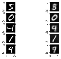
One of the reasons for the low quality is using a low number of neurons (300) within the dense layer. Another reason is using just 2 elements for representing all images. The quality might be increased by using more elements but this increases the size of the compressed data.

Another reason is not using convolutional layers at all. Dense layers are good for capturing the global properties from the images and the convolutional layers are good for the local properties. The result could be enhanced by adding some convolutional layers.

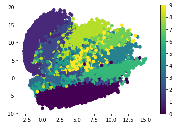
To have a better understanding of the output of the encoder model, let's display all the 1D vectors it returns according to the next code.

matplotlib.pyplot.figure()
matplotlib.pyplot.scatter(encoded_images[:, 0], encoded_images[:, 1], c=y_train) 
matplotlib.pyplot.colorbar()

The plot generated by this code is shown below. Generally, you can see that the model is able to cluster the different images in different regions but there is overlap between the different clusters.

Complete Code

The complete code discussed in this tutorial is listed below.

import tensorflow.keras.layers
import tensorflow.keras.models
import tensorflow.keras.optimizers
import tensorflow.keras.datasets
import numpy
import matplotlib.pyplot

# Encoder
x = tensorflow.keras.layers.Input(shape=(784), name="encoder_input")

encoder_dense_layer1 = tensorflow.keras.layers.Dense(units=300, name="encoder_dense_1")(x)
encoder_activ_layer1 = tensorflow.keras.layers.LeakyReLU(name="encoder_leakyrelu_1")(encoder_dense_layer1)

encoder_dense_layer2 = tensorflow.keras.layers.Dense(units=2, name="encoder_dense_2")(encoder_activ_layer1)
encoder_output = tensorflow.keras.layers.LeakyReLU(name="encoder_output")(encoder_dense_layer2)

encoder = tensorflow.keras.models.Model(x, encoder_output, name="encoder_model")
encoder.summary()

# Decoder
decoder_input = tensorflow.keras.layers.Input(shape=(2), name="decoder_input")

decoder_dense_layer1 = tensorflow.keras.layers.Dense(units=300, name="decoder_dense_1")(decoder_input)
decoder_activ_layer1 = tensorflow.keras.layers.LeakyReLU(name="decoder_leakyrelu_1")(decoder_dense_layer1)

decoder_dense_layer2 = tensorflow.keras.layers.Dense(units=784, name="decoder_dense_2")(decoder_activ_layer1)
decoder_output = tensorflow.keras.layers.LeakyReLU(name="decoder_output")(decoder_dense_layer2)

decoder = tensorflow.keras.models.Model(decoder_input, decoder_output, name="decoder_model")
decoder.summary()

# Autoencoder
ae_input = tensorflow.keras.layers.Input(shape=(784), name="AE_input")
ae_encoder_output = encoder(ae_input)
ae_decoder_output = decoder(ae_encoder_output)

ae = tensorflow.keras.models.Model(ae_input, ae_decoder_output, name="AE")
ae.summary()

# RMSE
def rmse(y_true, y_predict):
    return tensorflow.keras.backend.mean(tensorflow.keras.backend.square(y_true-y_predict))

# AE Compilation
ae.compile(loss="mse", optimizer=tensorflow.keras.optimizers.Adam(lr=0.0005))

# Preparing MNIST Dataset
(x_train_orig, y_train), (x_test_orig, y_test) = tensorflow.keras.datasets.mnist.load_data()
x_train_orig = x_train_orig.astype("float32") / 255.0
x_test_orig = x_test_orig.astype("float32") / 255.0

x_train = numpy.reshape(x_train_orig, newshape=(x_train_orig.shape[0], numpy.prod(x_train_orig.shape[1:])))
x_test = numpy.reshape(x_test_orig, newshape=(x_test_orig.shape[0], numpy.prod(x_test_orig.shape[1:])))

# Training AE
ae.fit(x_train, x_train, epochs=20, batch_size=256, shuffle=True, validation_data=(x_test, x_test))

encoded_images = encoder.predict(x_train)
decoded_images = decoder.predict(encoded_images)
decoded_images_orig = numpy.reshape(decoded_images, newshape=(decoded_images.shape[0], 28, 28))

num_images_to_show = 5
for im_ind in range(num_images_to_show):
    plot_ind = im_ind*2 + 1
    rand_ind = numpy.random.randint(low=0, high=x_train.shape[0])
    matplotlib.pyplot.subplot(num_images_to_show, 2, plot_ind)
    matplotlib.pyplot.imshow(x_train_orig[rand_ind, :, :], cmap="gray")
    matplotlib.pyplot.subplot(num_images_to_show, 2, plot_ind+1)
    matplotlib.pyplot.imshow(decoded_images_orig[rand_ind, :, :], cmap="gray")

matplotlib.pyplot.figure()
matplotlib.pyplot.scatter(encoded_images[:, 0], encoded_images[:, 1], c=y_train)
matplotlib.pyplot.colorbar()

Conclusion

This tutorial introduced the deep learning generative model known as autoencoders. This model consists of two building blocks: the encoder, and the decoder. The former encodes the input data as 1-D vectors, which are then to be decoded to reconstruct the original data. We saw how to apply this model using Keras to compress images from the MNIST dataset in twapplied the autoencoder using Keras for compressing the MNIST dataset in just 2 elements.